Robustness
Preliminaries: instantiation and execution of the MDO scenario
Let’s start with the following code lines which instantiate and execute the MDOScenario :
from gemseo.api import create_discipline, create_scenario

formulation = 'MDF'

disciplines = create_discipline(["SobieskiPropulsion", "SobieskiAerodynamics",
                                 "SobieskiMission", "SobieskiStructure"])

scenario = create_scenario(disciplines,
                           formulation=formulation,
                           objective_name="y_4",
                           maximize_objective=True,
                           design_space="design_space.txt")

scenario.set_differentiation_method("user")

algo_options = {'max_iter': 10, 'algo': "SLSQP"}
for constraint in ["g_1","g_2","g_3"]:
    scenario.add_constraint(constraint, 'ineq')

scenario.execute(algo_options)
Robustness
Description
The Robustness post processing
performs a quadratic approximation from an optimization history,
and plot the results as cuts of the approximation
computes the quadratic approximations of all the output functions,
propagate analytically a normal distribution centered on the optimal
design variable with a standard deviation which is a percentage
of the mean passed in option (default: 1%)
and plot the corresponding output boxplot.
It is possible either to save the plot, to show the plot or both.
Options
extension,
str- file extensionfile_path,
str- the base paths of the files to exportsave,
bool- if True, exports plot to pdfshow,
bool- if True, displays the plot windowsstddev,
float- standard deviation of inputs as fraction of x bounds
Case of the MDF formulation
To plot the robustness, use the API method execute_post()
with the keyword “Robustness” and
additional arguments concerning the type of display (file, screen, both):
scenario.post_process(“Robustness”, save=True, show=False, file_path=“mdf”)
The robustness of the optimum is represented by a box plot. Using the quadratic approximations of all the output functions, we propagate analytically a normal distribution with 1% standard deviation on all the design variables, assuming no cross-correlations of inputs, to obtain the mean and standard deviation of the resulting normal distribution. 500 samples are randomly generated from the resulting distribution, whose quartiles are plotted, relatively to the values of the function at the optimum. For each function (in abscissa), the plot shows the extreme values encountered in the 500 samples (top and bottom bars). Then, 95% of the values are within the blue boxes. The average is given by the red bar.
Figure Robustness on the Sobieski use case for the MDF formulation gives a qualitative information on the robustness of the optimum. Here for instance, 95% of the perturbed designs have a range degraded by less than 10 miles out of 3947 miles at the SSBJ’s problem optimum, ie. 0.2%. At worse, the range is degraded by 40 miles, ie. 0.8%. Here, since the normal distribution was used (which is symmetrical), the average is not altered. Besides, the constraints values are not altered by the perturbations. Therefore, we can say that the optimum is relatively robust with respect to perturbation of 1% of standard deviation.
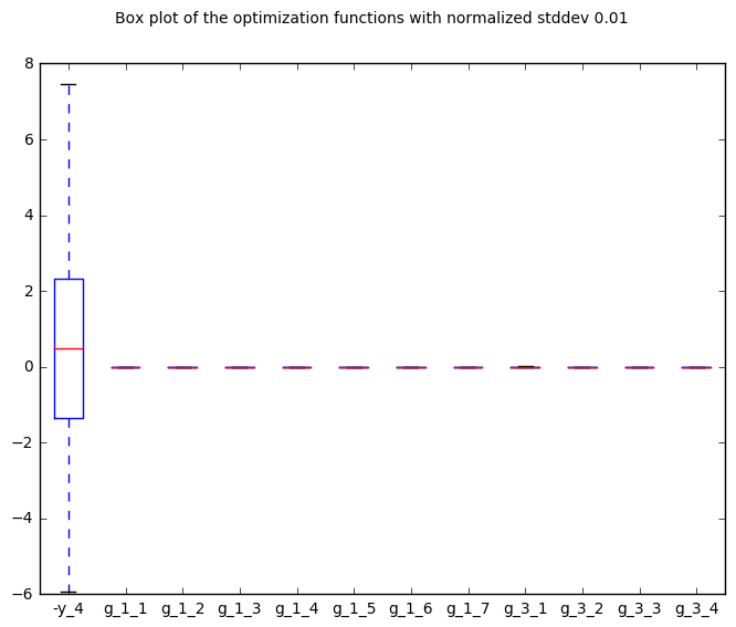
Robustness on the Sobieski use case for the MDF formulation