Note
Click here to download the full example code
Parameter space
In this example,
we will see the basics of ParameterSpace.
from matplotlib import pyplot as plt

from gemseo.algos.parameter_space import ParameterSpace
from gemseo.api import configure_logger, create_discipline, create_scenario

configure_logger()
Out:
<RootLogger root (INFO)>
Create a parameter space
Firstly,
the creation of a ParameterSpace does not require any mandatory argument:
parameter_space = ParameterSpace()
Out:
INFO - 09:23:59: *** Create a new parameter space ***
Then, we can add either deterministic variables
from their lower and upper bounds
(use ParameterSpace.add_variable())
or uncertain variables from their distribution names and parameters
(use ParameterSpace.add_random_variable())
parameter_space.add_variable("x", l_b=-2.0, u_b=2.0)
parameter_space.add_random_variable("y", "SPNormalDistribution", mu=0.0, sigma=1.0)
print(parameter_space)
Out:
    INFO - 09:23:59: Define the random variable: y
    INFO - 09:23:59:    Distribution: norm(mu=0.0, sigma=1.0)
    INFO - 09:23:59:    Dimension: 1
    INFO - 09:23:59: |_ Mathematical support: [array([-inf,  inf])]
    INFO - 09:23:59: |_ Numerical range: [array([-7.03448383,  7.03448691])]
    INFO - 09:23:59: Add the random variable: y
    INFO - 09:23:59: Define the random variable: y
    INFO - 09:23:59:    Distribution: Composed(independent_copula)
    INFO - 09:23:59:    Dimension: 1
    INFO - 09:23:59:    Marginals:
    INFO - 09:23:59:       y(1): norm(mu=0.0, sigma=1.0)
+----------------------------------------------------------------------------+
|                              Parameter space                               |
+------+-------------+-------+-------------+-------+-------------------------+
| name | lower_bound | value | upper_bound | type  |   Initial distribution  |
+------+-------------+-------+-------------+-------+-------------------------+
| x    |      -2     |  None |      2      | float |                         |
| y    |     -inf    |   0   |     inf     | float | norm(mu=0.0, sigma=1.0) |
+------+-------------+-------+-------------+-------+-------------------------+
We can check that the deterministic and uncertain variables are implemented as deterministic and deterministic variables respectively:
print("x is deterministic: ", parameter_space.is_deterministic("x"))
print("y is deterministic: ", parameter_space.is_deterministic("y"))
print("x is uncertain: ", parameter_space.is_uncertain("x"))
print("y is uncertain: ", parameter_space.is_uncertain("y"))
Out:
x is deterministic:  True
y is deterministic:  False
x is uncertain:  False
y is uncertain:  True
Sample from the parameter space
We can sample the uncertain variables from the ParameterSpace
and get values either as a NumPy array (by default)
or as a dictionary of NumPy arrays indexed by the names of the variables:
sample = parameter_space.compute_samples(n_samples=2, as_dict=True)
print(sample)
sample = parameter_space.compute_samples(n_samples=4)
print(sample)
Out:
[{'y': array([-1.01701414])}, {'y': array([0.63736181])}]
[[-0.85990661]
 [ 1.77260763]
 [-1.11036305]
 [ 0.18121427]]
Sample a discipline over the parameter space
We can also sample a discipline over the parameter space.
For simplicity,
we instantiate an AnalyticDiscipline from a dictionary of expressions:
discipline = create_discipline("AnalyticDiscipline", expressions_dict={"z": "x+y"})
From these parameter space and discipline,
we build a DOEScenario
and execute it with a Latin Hypercube Sampling algorithm and 100 samples.
Warning
A DOEScenario considers all the variables
available in its DesignSpace.
By inheritance,
in the special case of a ParameterSpace,
a DOEScenario considers all the variables
available in this ParameterSpace.
Thus,
if we do not filter the uncertain variables,
the DOEScenario will consider
both the deterministic variables as uniformly distributed variables
and the uncertain variables with their specified probability distributions.
scenario = create_scenario(
    [discipline], "DisciplinaryOpt", "z", parameter_space, scenario_type="DOE"
)
scenario.execute({"algo": "lhs", "n_samples": 100})
Out:
    INFO - 09:23:59:
    INFO - 09:23:59: *** Start DOE Scenario execution ***
    INFO - 09:23:59: DOEScenario
    INFO - 09:23:59:    Disciplines: AnalyticDiscipline
    INFO - 09:23:59:    MDOFormulation: DisciplinaryOpt
    INFO - 09:23:59:    Algorithm: lhs
    INFO - 09:23:59: Optimization problem:
    INFO - 09:23:59:    Minimize: z(x, y)
    INFO - 09:23:59:    With respect to: x, y
    INFO - 09:23:59: DOE sampling:   0%|          | 0/100 [00:00<?, ?it]
    INFO - 09:23:59: DOE sampling:  69%|██████▉   | 69/100 [00:00<00:00, 986.94 it/sec, obj=-3.33]
    INFO - 09:23:59: DOE sampling: 100%|██████████| 100/100 [00:00<00:00, 679.66 it/sec, obj=-2.21]
    INFO - 09:23:59: Optimization result:
    INFO - 09:23:59: Objective value = -3.3284373246961634
    INFO - 09:23:59: The result is feasible.
    INFO - 09:23:59: Status: None
    INFO - 09:23:59: Optimizer message: None
    INFO - 09:23:59: Number of calls to the objective function by the optimizer: 100
    INFO - 09:23:59: +-----------------------------------------------------------------------------------------+
    INFO - 09:23:59: |                                     Parameter space                                     |
    INFO - 09:23:59: +------+-------------+--------------------+-------------+-------+-------------------------+
    INFO - 09:23:59: | name | lower_bound |       value        | upper_bound | type  |   Initial distribution  |
    INFO - 09:23:59: +------+-------------+--------------------+-------------+-------+-------------------------+
    INFO - 09:23:59: | x    |      -2     | -1.959995425007306 |      2      | float |                         |
    INFO - 09:23:59: | y    |     -inf    | -1.368441899688857 |     inf     | float | norm(mu=0.0, sigma=1.0) |
    INFO - 09:23:59: +------+-------------+--------------------+-------------+-------+-------------------------+
    INFO - 09:23:59: *** DOE Scenario run terminated ***

{'eval_jac': False, 'algo': 'lhs', 'n_samples': 100}
We can export the optimization problem to a Dataset:
dataset = scenario.formulation.opt_problem.export_to_dataset(name="samples")
and visualize it in a tabular way:
print(dataset.export_to_dataframe())
Out:
   design_parameters           functions
                   x         y         z
                   0         0         0
0           1.869403  1.246453  3.115855
1          -1.567970  3.285041  1.717071
2           0.282640 -0.101706  0.180934
3           1.916313  1.848317  3.764630
4           1.562653  0.586038  2.148691
..               ...       ...       ...
95          0.120633 -0.327477 -0.206844
96         -0.999225  1.461403  0.462178
97         -1.396066 -0.972779 -2.368845
98          1.090093  0.225565  1.315658
99         -1.433207 -0.779330 -2.212536

[100 rows x 3 columns]
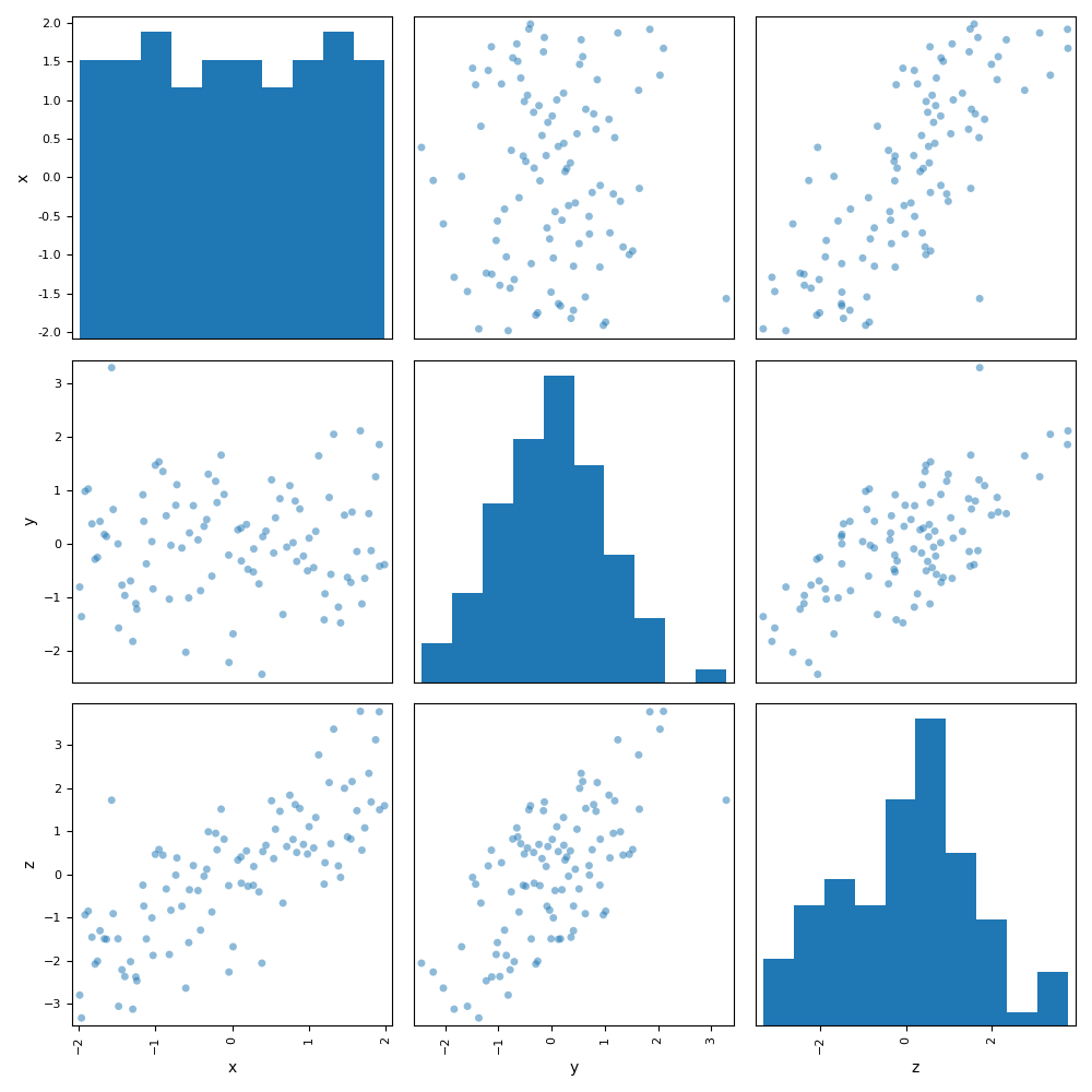
or with a graphical post-processing, e.g. a scatter plot matrix:
dataset.plot("ScatterMatrix", show=False)
# Workaround for HTML rendering, instead of ``show=True``
plt.show()
Sample a discipline over the uncertain space
If we want to sample a discipline over the uncertain space, we need to extract it:
uncertain_space = parameter_space.extract_uncertain_space()
Then, we clear the cache, create a new scenario from this parameter space containing only the uncertain variables and execute it.
discipline.cache.clear()
scenario = create_scenario(
    [discipline], "DisciplinaryOpt", "z", uncertain_space, scenario_type="DOE"
)
scenario.execute({"algo": "lhs", "n_samples": 100})
Out:
    INFO - 09:24:00:
    INFO - 09:24:00: *** Start DOE Scenario execution ***
    INFO - 09:24:00: DOEScenario
    INFO - 09:24:00:    Disciplines: AnalyticDiscipline
    INFO - 09:24:00:    MDOFormulation: DisciplinaryOpt
    INFO - 09:24:00:    Algorithm: lhs
    INFO - 09:24:00: Optimization problem:
    INFO - 09:24:00:    Minimize: z(y)
    INFO - 09:24:00:    With respect to: y
    INFO - 09:24:00: DOE sampling:   0%|          | 0/100 [00:00<?, ?it]
    INFO - 09:24:00: DOE sampling:  73%|███████▎  | 73/100 [00:00<00:00, 987.94 it/sec, obj=-.34]
    INFO - 09:24:00: DOE sampling: 100%|██████████| 100/100 [00:00<00:00, 715.11 it/sec, obj=-.813]
    INFO - 09:24:00: Optimization result:
    INFO - 09:24:00: Objective value = -2.6379682068246657
    INFO - 09:24:00: The result is feasible.
    INFO - 09:24:00: Status: None
    INFO - 09:24:00: Optimizer message: None
    INFO - 09:24:00: Number of calls to the objective function by the optimizer: 100
    INFO - 09:24:00: +-----------------------------------------------------------------------------------------+
    INFO - 09:24:00: |                                     Parameter space                                     |
    INFO - 09:24:00: +------+-------------+--------------------+-------------+-------+-------------------------+
    INFO - 09:24:00: | name | lower_bound |       value        | upper_bound | type  |   Initial distribution  |
    INFO - 09:24:00: +------+-------------+--------------------+-------------+-------+-------------------------+
    INFO - 09:24:00: | y    |     -inf    | -2.637968206824666 |     inf     | float | norm(mu=0.0, sigma=1.0) |
    INFO - 09:24:00: +------+-------------+--------------------+-------------+-------+-------------------------+
    INFO - 09:24:00: *** DOE Scenario run terminated ***

{'eval_jac': False, 'algo': 'lhs', 'n_samples': 100}
Finally, we build a dataset from the disciplinary cache and visualize it. We can see that the deterministic variable ‘x’ is set to its default value for all evaluations, contrary to the previous case where we were considering the whole parameter space:
dataset = scenario.formulation.opt_problem.export_to_dataset(name="samples")
print(dataset.export_to_dataframe())
Out:
   design_parameters functions
                   y         z
                   0         0
0          -0.640726 -0.640726
1          -0.393653 -0.393653
2           0.550565  0.550565
3           0.944369  0.944369
4          -2.115275 -2.115275
..               ...       ...
95          0.081947  0.081947
96         -1.085812 -1.085812
97         -0.761651 -0.761651
98         -0.042932 -0.042932
99         -0.813354 -0.813354

[100 rows x 2 columns]
Total running time of the script: ( 0 minutes 1.219 seconds)