Correlations
Preliminaries: instantiation and execution of the MDO scenario
Let’s start with the following code lines which instantiate and execute the MDOScenario :
from gemseo.api import create_discipline, create_scenario

formulation = 'MDF'

disciplines = create_discipline(["SobieskiPropulsion", "SobieskiAerodynamics",
                                 "SobieskiMission", "SobieskiStructure"])

scenario = create_scenario(disciplines,
                           formulation=formulation,
                           objective_name="y_4",
                           maximize_objective=True,
                           design_space="design_space.txt")

scenario.set_differentiation_method("user")

algo_options = {'max_iter': 10, 'algo': "SLSQP"}
for constraint in ["g_1","g_2","g_3"]:
    scenario.add_constraint(constraint, 'ineq')

scenario.execute(algo_options)
Correlations
Description
A correlation coefficient indicates whether there is a linear relationship between 2 quantities \(x\) and \(y\), in which case it equals 1 or -1. It is the normalized covariance between the two quantities:
The Correlations post processing builds scatter plots of correlated variables among design variables, output functions, and constraints.
The plot method considers all variable correlations greater than 95%. A different threshold value and/or a sublist of variable names can be passed as options. The x- and y-figure sizes can also be modified in options. It is possible to either save the plot, to show the plot or both.
Options
func_names,
list(str)- The func_names for which the correlations are computed. If None, all functions are considered.coeff_limit,
float- If the correlation between the variables is lower than coeff_limit, the plot is not made.n_plots_x,
int- The number of horizontal plots.n_plots_y,
int- The number of vertical plots.save,
bool- If True, export the plot to file.show,
bool- If True, display the plot windows.file_path,
str- The base paths of the files to export. If None, use the current working directory.extension,
str- The file extension.figsize_x,
int- The size of the figure in the horizontal direction (inches).figsize_y,
int- The size of figure in the vertical direction (inches).
Case of the MDF formulation
To compute the correlations between all inputs and all outputs as well
as between two outputs, use the API method execute_post()
with the keyword "Correlations" and
additional arguments concerning the type of display (file, screen, both):
scenario.post_process("Correlations", coeff_limit=0.85, save=True,
show=False, n_plots_x=4, n_plots_y=4)
where:
coeff_limitis the absolute threshold for correlation plots. It filters the minimum correlation coefficient to be displayed,n_plot_xandn_plot_yare the numbers of plots along the columns and the rows, respectively.
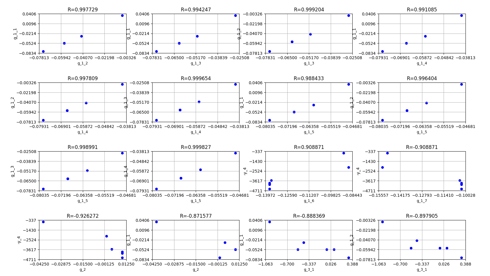
Correlation coefficients on the Sobieski use case for the MDF formulation
As mentioned earlier, correlation plots highlight the strong correlations between stress constraints in wing sections : the correlation coefficients belong to \([0.94766, 0.999286]\).
The aerodynamics constraint g_2 is a polynomial function of
\(x_1\): \(g\_2=1+0.2\overline{x_1}\) with
\(\overline{x_1}\) the normalized value of \(x_1\).