History of evaluations¶

Preliminaries: instantiation and execution of the MDO scenario¶

Let’s start with the following code lines which instantiate and execute the MDOScenario :

from gemseo.api import create_discipline, create_scenario

formulation = 'MDF'

disciplines = create_discipline(["SobieskiPropulsion", "SobieskiAerodynamics",
                                 "SobieskiMission", "SobieskiStructure"])

scenario = create_scenario(disciplines,
                           formulation=formulation,
                           objective_name="y_4",
                           maximize_objective=True,
                           design_space="design_space.txt")

scenario.set_differentiation_method("user")

algo_options = {'max_iter': 10, 'algo': "SLSQP"}
for constraint in ["g_1","g_2","g_3"]:
    scenario.add_constraint(constraint, 'ineq')

scenario.execute(algo_options)

OptHistoryView¶

Description¶

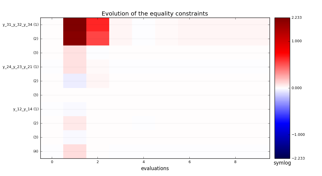
The OptHistoryView post processing performs separated plots: the design variables history, the objective function history, the history of hessian approximation of the objective, the inequality constraint history, the equality constraint history, and constraints histories.

By default, all design variables are considered. A sublist of design variables can be passed as options. Minimum and maximum values for the plot can be passed as options. The objective function can also be represented in terms of difference w.r.t. the initial value It is possible either to save the plot, to show the plot or both.

Options¶

extension, str - file extension
file_path, str - the base paths of the files to export
obj_max, float - maximum value for the objective in the plot
obj_min, float - minimum value for the objective in the plot
obj_relative, bool - plot the objective value difference with the initial value
save, bool - if True, exports plot to pdf
show, bool - if True, displays the plot windows
variables_names, list(str) - list of the names of the variables to display

This post-processing feature is illustrated on the scenario.

Case of the MDF formulation¶

To visualize the optimization history of the scenario, we use the execute_post() API method with the keyword "OptHistoryView" and additional arguments concerning the type of display (file, screen, both):

scenario.post_process("OptHistoryView", save=True, show=False,
                      file_path="mdf", extension="png")

This triggers the creation of five plots.

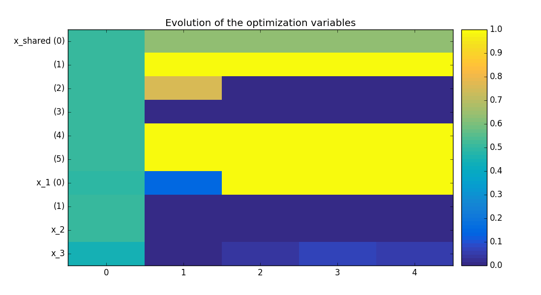
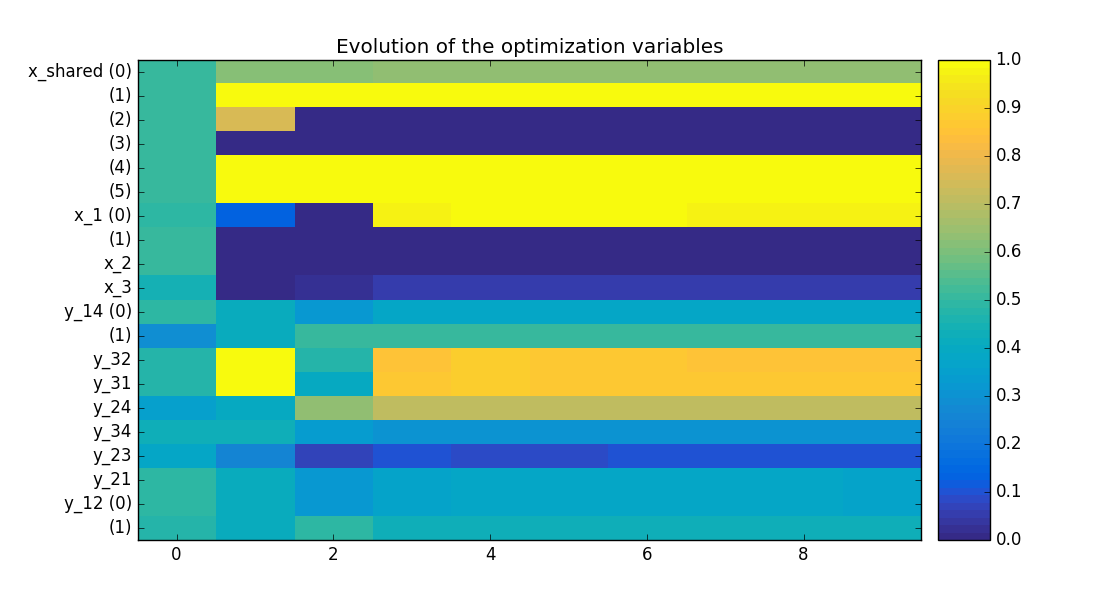
mdf_variables_history.png - The first graph shows the normalized values of the design variables, the \(y\) axis is the index of the inputs in the vector; and the \(x\) axis represents the iterations.

Design variables history on the Sobieski use case for the MDF formulation¶

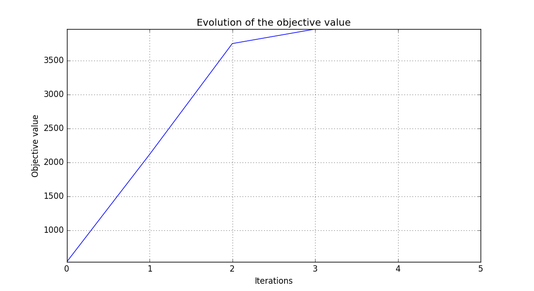
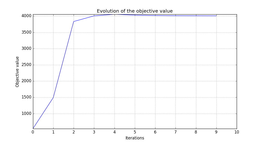
mdf_obj_history.png - The second graph shows the evolution of the objective value during the optimization.

Objective function history on the Sobieski use case for the MDF formulation¶
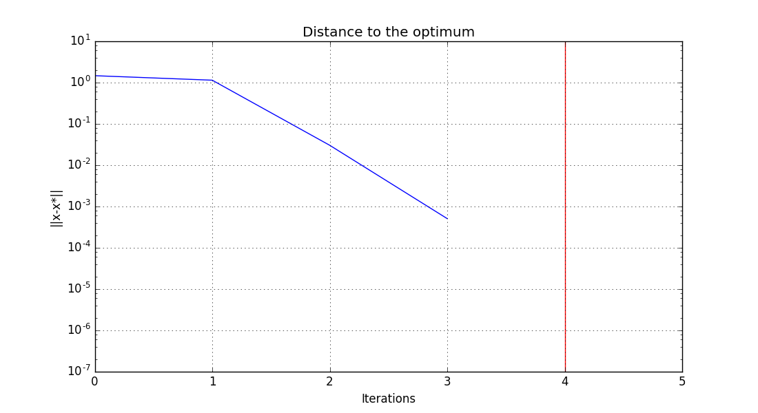
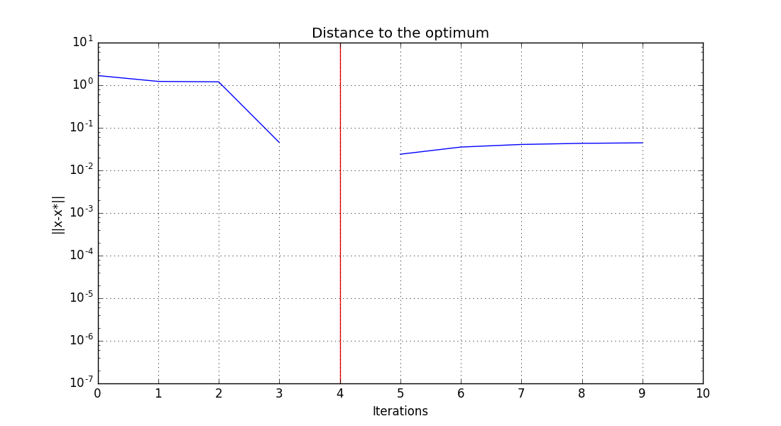
mdf_x_xstar_history.png - The third graph plots the distance to the best design variables vector in log scale \(log( ||x-x^*|| )\).

Distance to the optimum history on the Sobieski use case for the MDF formulation¶
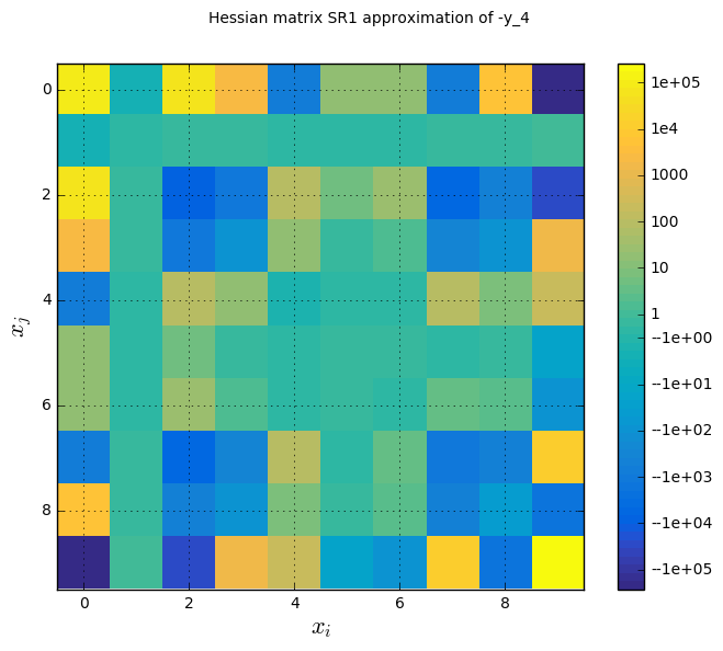
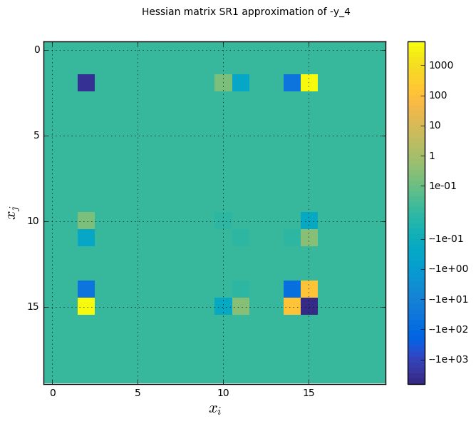
mdf_hessian_approx.png - The fourth graph shows an approximation of the second order derivatives of the objective function \(\frac{\partial^2 f(x)}{\partial x^2}\), which is a measure of the sensitivity of the function with respect to the design variables, and of the anisotropy of the problem (differences of curvatures in the design space).

Hessian diagonal approximation history on the Sobieski use case for the MDF formulation¶
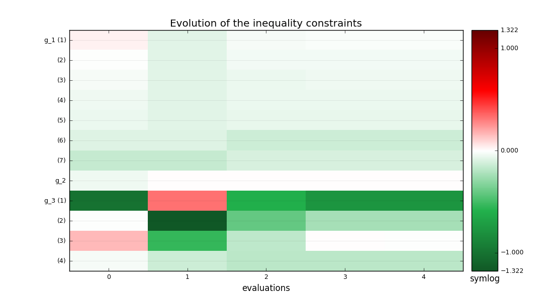
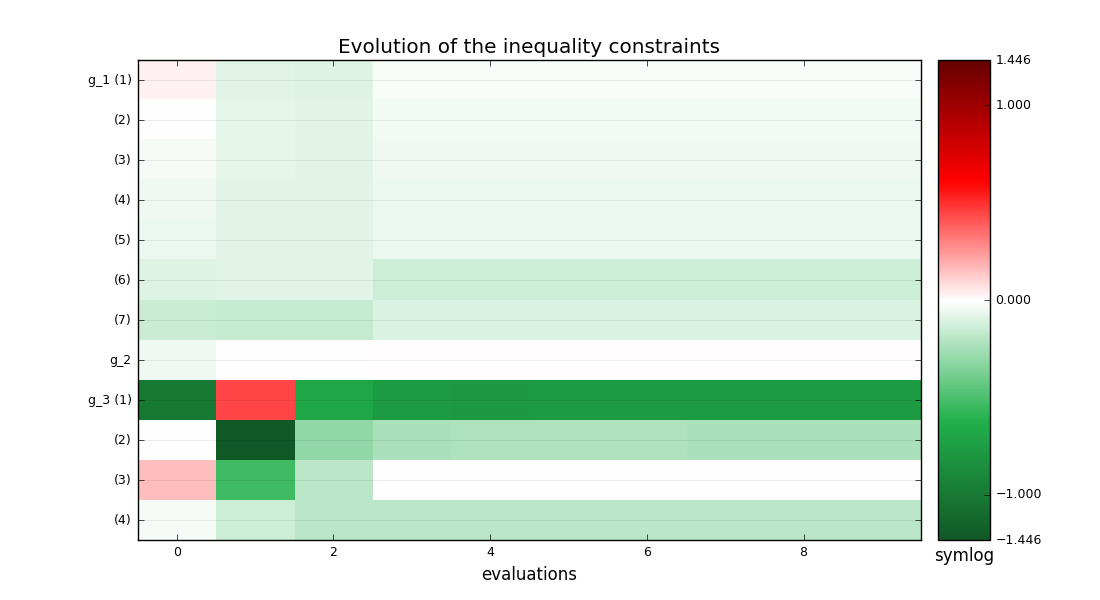
mdf_ineq_constraints_history.png - The last graph portrays the evolution of the values of the constraints. The components of \(g\_1, g\_2, g\_3\) are concatenated as a single vector of size 12. The constraints must be non-positive, that is the plot must be green or white for satisfied (white = active, red = violated). At convergence, only two are active.

History of the constraints on the Sobieski use case for the MDF formulation¶

Case of the IDF formulation¶

Now, if we consider the IDF formulation, after the execution of scenario, the optimization history may be visualized:

scenario.post_process("OptHistoryView", save=True, show=False,
                      file_path="idf", extension="png")

This triggers the creation of six plots.

idf_variables_history.png - The first graph shows the normalized values of the design variables, the \(y\) axis is the index of the inputs in the vector; and the \(x\) axis represents the iterations. Compared to MDF, additional variables (indices 10 to 20), generated by the formulation, occur in the consistency .

Design variables history on the Sobieski use case for the IDF formulation¶
idf_obj_history.png - The second graph shows the evolution of the objective value during the optimization.

Objective function history on the Sobieski use case for the IDF formulation¶
idf_x_xstar_history.png - The third graph plots the distance to the best design variables vector in log scale \(log( ||x-x^*|| )\).

Distance to the optimum history on the Sobieski use case for the IDF formulation.¶
idf_hessian_approx.png - The fourth graph shows an approximation of the second order derivatives of the objective function \(\frac{\partial^2 f(x)}{\partial x^2}\), which is a measure of the sensitivity of the function with respect to the design variables, and of the anisotropy of the problem (differences of curvatures in the design space).

Hessian diagonal approximation history on the Sobieski use case for the IDF formulation¶
mdf_ineq_constraints_history.png - The last graphs portray the evolution of the values of the constraints. Figures History of the inequality constraints on the Sobieski use case for the IDF formulation and History of the equality constraints on the Sobieski use case for the IDF formulation portray the evolution of the values of the inequality and equality constraints, respectively. The components of g_1, g_2, g_3 are concatenated as a single vector of size 12. The inequality constraints must be non-positive, that is the plot must be green or white for satisfied constraints (white = active, red = violated). At convergence, only two inequality constraints are active.

History of the inequality constraints on the Sobieski use case for the IDF formulation¶

History of the equality constraints on the Sobieski use case for the IDF formulation¶