Scalable problem of Tedford and Martins, 2010

from __future__ import division, unicode_literals

from numpy import array
from numpy.random import rand

from gemseo.api import configure_logger, generate_n2_plot
from gemseo.problems.scalable.parametric.core.design_space import TMDesignSpace
from gemseo.problems.scalable.parametric.disciplines import (
    TMMainDiscipline,
    TMSubDiscipline,
)
from gemseo.problems.scalable.parametric.problem import TMScalableProblem
from gemseo.problems.scalable.parametric.study import (
    TMParamSS,
    TMParamSSPost,
    TMScalableStudy,
)

configure_logger()

Disciplines

We define two strongly coupled disciplines and a weakly coupled discipline, with:

• 2 shared design parameters,

• 2 local design parameters for the first discipline,

• 3 local design parameters for the second discipline,

• 3 coupling variables for the first discipline,

• 2 coupling variables for the second discipline.

sizes = {"x_shared": 2, "x_local_0": 2, "x_local_1": 3, "y_0": 3, "y_1": 2}

We use any values for the coefficients and the default values of the design parameters and coupling variables.

Strongly coupled disciplines

Here is the first strongly coupled discipline.

default_inputs = {
    "x_shared": rand(sizes["x_shared"]),
    "x_local_0": rand(sizes["x_local_0"]),
    "y_1": rand(sizes["y_1"]),
}
index = 0
c_shared = rand(sizes["y_0"], sizes["x_shared"])
c_local = rand(sizes["y_0"], sizes["x_local_0"])
c_coupling = {"y_1": rand(sizes["y_0"], sizes["y_1"])}
disc0 = TMSubDiscipline(index, c_shared, c_local, c_coupling, default_inputs)

print(disc0.name)
print(disc0.get_input_data_names())
print(disc0.get_output_data_names())

TM_Discipline_0
dict_keys(['x_shared', 'x_local_0', 'y_1'])
dict_keys(['y_0'])

Here is the second one, strongly coupled with the first one.

default_inputs = {
    "x_shared": rand(sizes["x_shared"]),
    "x_local_1": rand(sizes["x_local_1"]),
    "y_0": rand(sizes["y_0"]),
}
index = 1
c_shared = rand(sizes["y_1"], sizes["x_shared"])
c_local = rand(sizes["y_1"], sizes["x_local_1"])
c_coupling = {"y_0": rand(sizes["y_1"], sizes["y_0"])}
disc1 = TMSubDiscipline(index, c_shared, c_local, c_coupling, default_inputs)

print(disc1.name)
print(disc1.get_input_data_names())
print(disc1.get_output_data_names())

TM_Discipline_1
dict_keys(['x_shared', 'x_local_1', 'y_0'])
dict_keys(['y_1'])

Weakly coupled discipline

Here is the discipline weakly coupled to the previous ones.

c_constraint = [array([1.0, 2.0]), array([3.0, 4.0, 5.0])]
default_inputs = {
    "x_shared": array([0.5]),
    "y_0": array([2.0, 3.0]),
    "y_1": array([4.0, 5.0, 6.0]),
}
system = TMMainDiscipline(c_constraint, default_inputs)

print(system.name)
print(system.get_input_data_names())
print(system.get_output_data_names())

TM_System
dict_keys(['x_shared', 'y_0', 'y_1'])
dict_keys(['obj', 'cstr_0', 'cstr_1'])

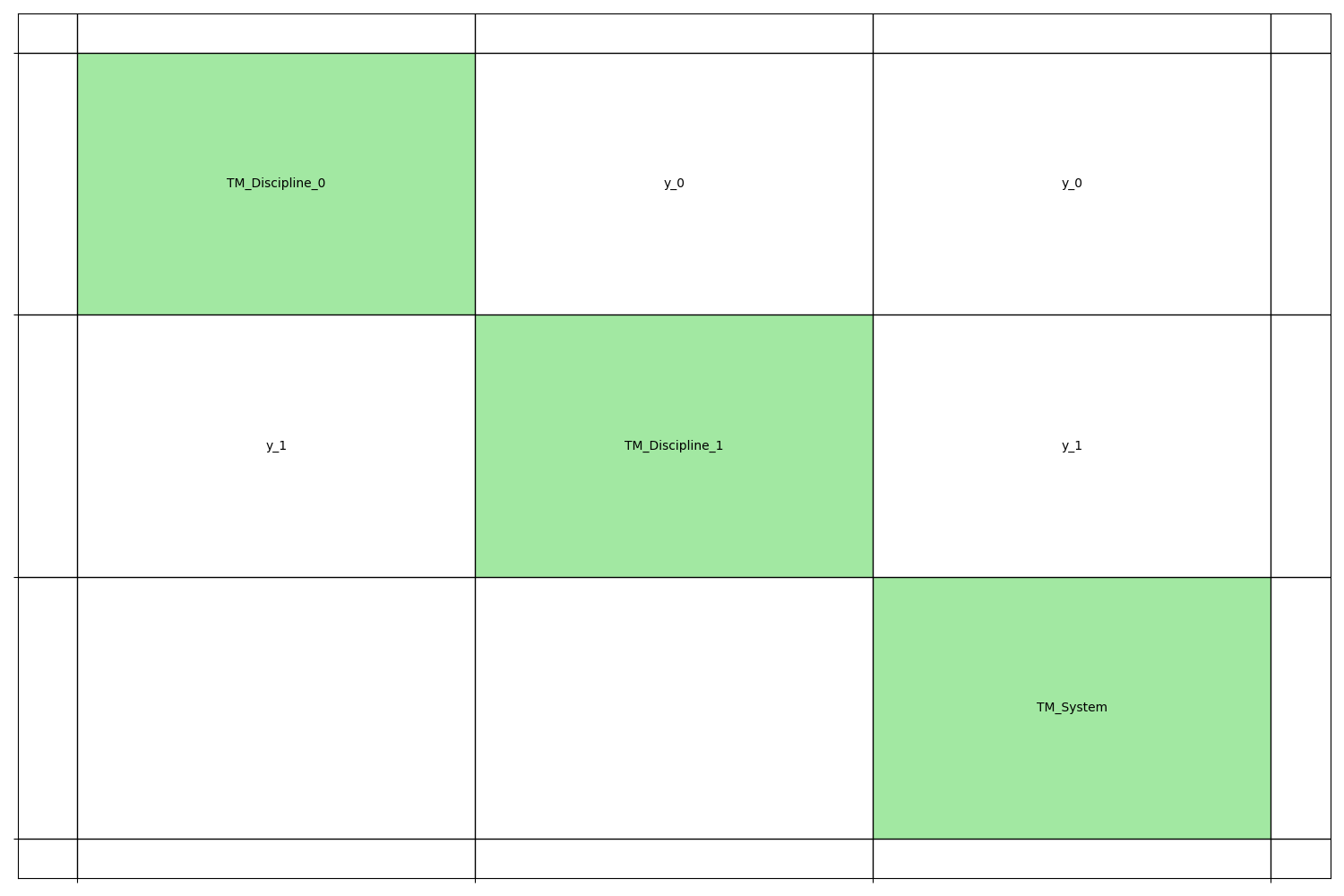
Coupling chart

We can represent these three disciplines by means of an N2 chart.

generate_n2_plot([disc0, disc1, system], save=False, show=True)

Design space

We define the design space from the sizes of the shared design parameters, local parameters and coupling variables.

n_shared = sizes["x_shared"]
n_local = [sizes["x_local_0"], sizes["x_local_1"]]
n_coupling = [sizes["y_0"], sizes["y_1"]]
design_space = TMDesignSpace(n_shared, n_local, n_coupling)

print(design_space)

Design Space:
+-----------+-------------+-------+-------------+-------+
| name      | lower_bound | value | upper_bound | type  |
+-----------+-------------+-------+-------------+-------+
| x_local_0 |      0      |  0.5  |      1      | float |
| x_local_0 |      0      |  0.5  |      1      | float |
| x_local_1 |      0      |  0.5  |      1      | float |
| x_local_1 |      0      |  0.5  |      1      | float |
| x_local_1 |      0      |  0.5  |      1      | float |
| x_shared  |      0      |  0.5  |      1      | float |
| x_shared  |      0      |  0.5  |      1      | float |
| y_0       |      0      |  0.5  |      1      | float |
| y_0       |      0      |  0.5  |      1      | float |
| y_0       |      0      |  0.5  |      1      | float |
| y_1       |      0      |  0.5  |      1      | float |
| y_1       |      0      |  0.5  |      1      | float |
+-----------+-------------+-------+-------------+-------+

Scalable problem

We define a scalable problem based on two strongly coupled disciplines and a weakly one, with the following properties:

• 3 shared design parameters,

• 2 local design parameters for the first strongly coupled discipline,

• 2 coupling variables for the first strongly coupled discipline,

• 4 local design parameters for the second strongly coupled discipline,

• 3 coupling variables for the second strongly coupled discipline.

problem = TMScalableProblem(3, [2, 4], [2, 3])

print(problem)

print(problem.get_design_space())

print(problem.get_default_inputs())

Scalable problem
> TM_System
   >> Inputs:
      | x_shared (3)
      | y_0 (2)
      | y_1 (3)
   >> Outputs:
      | cstr_0 (2)
      | cstr_1 (3)
      | obj (1)
> TM_Discipline_0
   >> Inputs:
      | x_local_0 (2)
      | x_shared (3)
      | y_1 (3)
   >> Outputs:
      | y_0 (2)
> TM_Discipline_1
   >> Inputs:
      | x_local_1 (4)
      | x_shared (3)
      | y_0 (2)
   >> Outputs:
      | y_1 (3)

Design Space:
+-----------+-------------+-------+-------------+-------+
| name      | lower_bound | value | upper_bound | type  |
+-----------+-------------+-------+-------------+-------+
| x_local_0 |      0      |  0.5  |      1      | float |
| x_local_0 |      0      |  0.5  |      1      | float |
| x_local_1 |      0      |  0.5  |      1      | float |
| x_local_1 |      0      |  0.5  |      1      | float |
| x_local_1 |      0      |  0.5  |      1      | float |
| x_local_1 |      0      |  0.5  |      1      | float |
| x_shared  |      0      |  0.5  |      1      | float |
| x_shared  |      0      |  0.5  |      1      | float |
| x_shared  |      0      |  0.5  |      1      | float |
| y_0       |      0      |  0.5  |      1      | float |
| y_0       |      0      |  0.5  |      1      | float |
| y_1       |      0      |  0.5  |      1      | float |
| y_1       |      0      |  0.5  |      1      | float |
| y_1       |      0      |  0.5  |      1      | float |
+-----------+-------------+-------+-------------+-------+
{'x_shared': array([0.5, 0.5, 0.5]), 'x_local_0': array([0.5, 0.5]),
'y_0': array([0.5, 0.5]), 'cstr_0': array([0.5]), 'x_local_1':
array([0.5, 0.5, 0.5, 0.5]), 'y_1': array([0.5, 0.5, 0.5]), 'cstr_1':
array([0.5])}

Scalable study

We define a scalable study based on two strongly coupled disciplines and a weakly one, with the following properties:

• 3 shared design parameters,

• 2 local design parameters for each strongly coupled discipline,

• 3 coupling variables for each strongly coupled discipline.

study = TMScalableStudy(n_disciplines=2, n_shared=3, n_local=2, n_coupling=3)
print(study)

Scalable study
> 2 disciplines
> 3 shared design parameters
> 2 local design parameters per discipline
> 3 coupling variables per discipline

Then, we run MDF and IDF formulations:

study.run_formulation("MDF")
study.run_formulation("IDF")

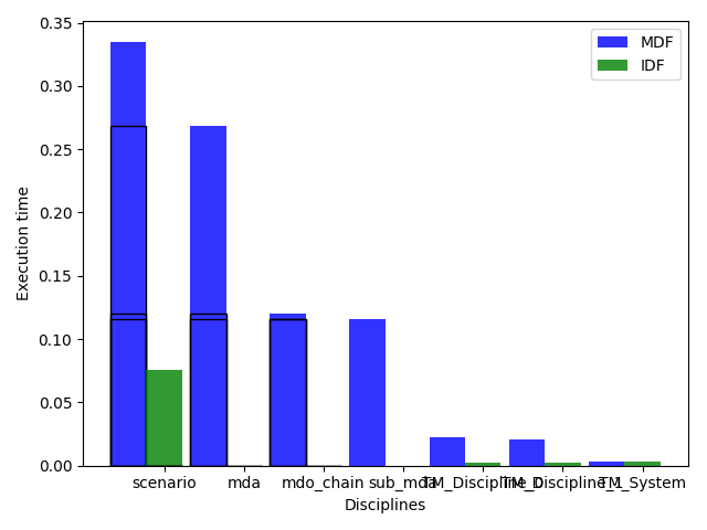
We can look at the result in the console:

print(study)

Scalable study
> 2 disciplines
> 3 shared design parameters
> 2 local design parameters per discipline
> 3 coupling variables per discipline

MDO formulations
> MDF
   >> TM_System = 9 calls / 7 linearizations / 3.29e-03 seconds
   >> TM_Discipline_0 = 132 calls / 7 linearizations / 2.19e-02 seconds
   >> TM_Discipline_1 = 124 calls / 7 linearizations / 2.04e-02 seconds
   >> mda = 7 calls / 7 linearizations / 2.68e-01 seconds
   >> mdo_chain = 7 calls / 0 linearizations / 1.20e-01 seconds
   >> sub_mda = 7 calls / 0 linearizations / 1.16e-01 seconds
   >> scenario = 1 calls / 0 linearizations / 3.35e-01 seconds
> IDF
   >> TM_System = 12 calls / 9 linearizations / 2.98e-03 seconds
   >> TM_Discipline_0 = 12 calls / 9 linearizations / 2.19e-03 seconds
   >> TM_Discipline_1 = 11 calls / 9 linearizations / 2.01e-03 seconds
   >> mda = 0 calls / 0 linearizations / 0.00e+00 seconds
   >> mdo_chain = 0 calls / 0 linearizations / 0.00e+00 seconds
   >> sub_mda = 0 calls / 0 linearizations / 0.00e+00 seconds
   >> scenario = 1 calls / 0 linearizations / 7.60e-02 seconds

or plot the execution time:

study.plot_exec_time()

Parametric scalability study

We define a parametric scalability study based on two strongly coupled disciplines and a weakly one, with the following properties:

• 3 shared design parameters,

• 2 coupling variables for each strongly coupled discipline,

• 1, 5 or 25 local design parameters for each strongly coupled discipline,

study = TMParamSS(n_disciplines=2, n_shared=3, n_local=[1, 5, 25], n_coupling=2)
print(study)

Parametric scalable study
> 2 disciplines
> 3 shared design parameters
> 1, 5 or 25 local design parameters per discipline
> 2 coupling variables per discipline

Then, we run MDF and IDF formulations:

study.run_formulation("MDF")
study.run_formulation("IDF")

and save the results in a pickle file:

study.save("results.pkl")

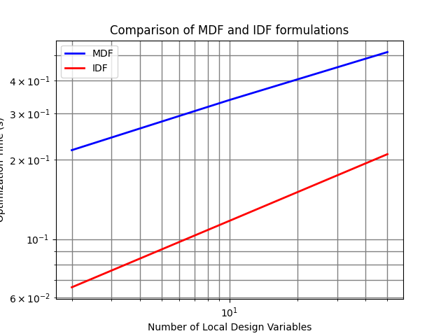
We can plot these results and compare MDF and IDF formulations in terms of execution time for different number of local design variables.

results = TMParamSSPost("results.pkl")
results.plot("Comparison of MDF and IDF formulations")