Note
Click here to download the full example code
Comparing sensitivity indices
from matplotlib import pyplot as plt
from numpy import pi

from gemseo.algos.parameter_space import ParameterSpace
from gemseo.api import create_discipline
from gemseo.uncertainty.sensitivity.correlation.analysis import CorrelationAnalysis
from gemseo.uncertainty.sensitivity.morris.analysis import MorrisAnalysis
In this example, we consider the Ishigami function:
which is well-known in the uncertainty domain:
expressions = {"y": "sin(x1)+7*sin(x2)**2+0.1*x3**4*sin(x1)"}
discipline = create_discipline(
    "AnalyticDiscipline", expressions_dict=expressions, name="Ishigami"
)
The different uncertain variables \(X_1\) , \(X_2\) and \(X_3\) are independent and identically distributed according to an uniform distribution between \(-\pi\) and \(\pi\):
space = ParameterSpace()
for variable in ["x1", "x2", "x3"]:
    space.add_random_variable(
        variable, "OTUniformDistribution", minimum=-pi, maximum=pi
    )
We would like to carry out two sensitivity analyses, e.g. a first one based on correlation coefficients and a second one based on the Morris methodology, and compare the results,
Firstly,
we create a CorrelationAnalysis
and compute the sensitivity indices:
correlation = CorrelationAnalysis(discipline, space, 10)
correlation.compute_indices()
Out:
{'pearson': {'y': [{'x1': array([0.68510393]), 'x2': array([0.64205033]), 'x3': array([-0.02179137])}]}, 'spearman': {'y': [{'x1': array([0.6]), 'x2': array([0.79393939]), 'x3': array([-0.05454545])}]}, 'pcc': {'y': [{'x1': array([0.47042845]), 'x2': array([0.379126]), 'x3': array([0.00273528])}]}, 'prcc': {'y': [{'x1': array([0.01882857]), 'x2': array([0.71401197]), 'x3': array([-0.34471095])}]}, 'src': {'y': [{'x1': array([0.22002806]), 'x2': array([0.12925357]), 'x3': array([3.7683822e-06])}]}, 'srrc': {'y': [{'x1': array([0.00024735]), 'x2': array([0.71116275]), 'x3': array([0.06229155])}]}, 'ssrrc': {'y': [{'x1': array([0.46907148]), 'x2': array([0.35951852]), 'x3': array([0.00194123])}]}}
Then,
we create a MorrisAnalysis
and compute the sensitivity indices:
morris = MorrisAnalysis(discipline, space, 10)
morris.compute_indices()
Out:
{'mu': {'y': [{'x1': array([-0.36000398]), 'x2': array([0.77781853]), 'x3': array([-0.70990541])}]}, 'mu_star': {'y': [{'x1': array([0.67947346]), 'x2': array([0.88906579]), 'x3': array([0.72694219])}]}, 'sigma': {'y': [{'x1': array([0.98724949]), 'x2': array([0.79064599]), 'x3': array([0.8074493])}]}, 'relative_sigma': {'y': [{'x1': array([1.45296254]), 'x2': array([0.88929976]), 'x3': array([1.11074761])}]}, 'min': {'y': [{'x1': array([0.0338188]), 'x2': array([0.11821721]), 'x3': array([8.72820113e-05])}]}, 'max': {'y': [{'x1': array([2.2360336]), 'x2': array([1.83987522]), 'x3': array([2.12052546])}]}}
Lastly,
we compare these analyses
with the graphical method SensitivityAnalysis.plot_comparison(),
either using a bar chart:
morris.plot_comparison(correlation, "y", use_bar_plot=True, save=False, show=False)
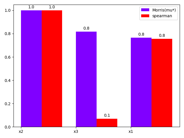
Out:
<gemseo.post.dataset.bars.BarPlot object at 0x7f618ffc2ee0>
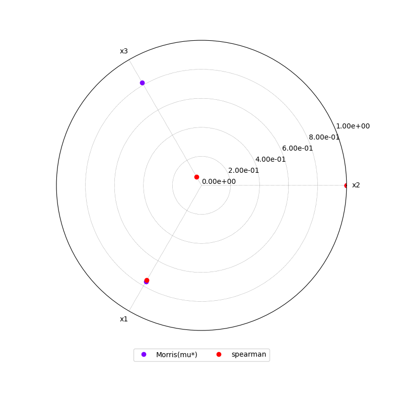
or a radar plot:
morris.plot_comparison(correlation, "y", use_bar_plot=False, save=False, show=False)
# Workaround for HTML rendering, instead of ``show=True``
plt.show()
Out:
/home/docs/checkouts/readthedocs.org/user_builds/gemseo/conda/3.2.0/lib/python3.8/site-packages/gemseo/post/dataset/dataset_plot.py:383: UserWarning: This figure includes Axes that are not compatible with tight_layout, so results might be incorrect.
  sub_figure.tight_layout()
Total running time of the script: ( 0 minutes 0.508 seconds)