Tutorial: How to carry out a trade-off study

This tutorial describes how to carry out a trade-off study by means of GEMSEO. For that, we consider the Sobieski problem.

Trade-off studies are implemented in the class DOEScenario.

All the post-processing tools presented in How to deal with post-processing for MDOScenario remain valid for trade-off studies, as well as the additional tools presented below.

Similarities between trade-off studies and optimization problems

Trade-off studies are supported by capabilities of Design Of Experiments. But, when comparing an optimization scenario and a trade-off scenario, similarities appear:

Feature	MDO Scenario (implemented in MDOScenario)	Trade-off study (implemented in DOEScenario)
Sample evaluation	The sample \(i+1\) requires the evaluation of the sample \(i\).	The sequence is defined a priori by a DOE; an iteration corresponds to a sample
Constraint and objective functions	They guide the convergence of an optimization problem.	They are only monitored evaluated outputs.
Constraint and objective functions	They are not directly outputs of a discipline.	They are not directly outputs of a discipline.
Constraint and objective functions	They can be computed by an Multi Disciplinary Analyses for instance (e.g. MDF)	They can be computed by an Multi Disciplinary Analyses for instance.
Constraint and objective functions	Target values can be used for the coupling variables (e.g. IDF).	Target values can be used for the coupling variables.

That is why in GEMSEO,

• the DOE sample evaluations are performed on the objective and constraint functions generated by an MDO formulation,

exactly as

• the optimization algorithm evaluates the objective and constraint functions to solve the optimization problem.

A key advantage of this approach is that the DOE is based on a formalized MDO problem.

Besides, from the implementation point of view, all existing methods developed for optimization can be used for trade-off without any change.

Finally, this smoothes the transition between a DOE study and an MDO study, and makes the DOE an ideal preparatory step for MDO.

Trade-offs based on a MDF formulation

As mentioned previously, a trade-off script and an optimization script are very similar. For example, a MDF trade-off study includes an Multi Disciplinary Analyses sampling with respect to the design variables provided by the DOE algorithm.

1. Define the MDODiscipline

We first instantiate the MDODiscipline:

from gemseo.api import create_discipline

disciplines = create_discipline(["SobieskiPropulsion", "SobieskiAerodynamics",
                                 "SobieskiMission", "SobieskiStructure"])

2. Define the DesignSpace

Then, by means of the API function read_design_space(), we load the DesignSpace, like for MDOScenario.

from gemseo.api import read_design_space

input_file = join(dirname(__file__), "sobieski_design_space.txt")
design_space = read_design_space(input_file)

3. Define the trade-off study

Initialization

The MDF formulation is selected to build the DOEScenario, like for MDOScenario.

from gemseo.api import create_scenario

scenario = create_scenario(disciplines,
                           formulation="MDF",
                           objective_name="y_4",
                           design_space=design_space,
                           scenario_type="DOE",
                           maximize_objective=True)

Constraint monitoring

We choose here to monitor the constraints, similarly to the MDO study:

for constraint in ["g_1", "g_2", "g_3"]:
    scenario.add_constraint(constraint, 'ineq')

This is optional since the driver is not able to ensure these constraints, but it is the only way to observe an output which is not an objective, in order to benefit from the post processing plots associated to these constraints. Besides, this does not increase the cost of the scenario execution, since the constraints are computed by the Sobieski disciplines in all cases, and a buffer system in avoids to call twice a discipline in a row with identical inputs, and directly returns the buffered outputs.

Optimization options

The DOE algorithm options are passed as inputs of the MDOScenario. The number of samples is specified, as well as the “criterion” option which is the center option of pyDOE centering the points within the sampling intervals. The sensitivity of the outputs with respect to the design variables may be computed, thanks to the coupled derivatives capabilities, to this aim the ‘eval_jac’ option is set to True.

doe_options = {'n_samples': 30,
               'algo': 'lhs',
               'eval_jac': True,
               'algo_options': {"criterion": "center"}}

See also

In this tutorial, the design is based on LHS from pyDOE, however, several other designs are available, based on the package or OpenTURNS. Some examples of these designs are plotted in DOE algorithms.

To list the available DOE algorithms in the current GEMSEO configuration, use gemseo.api.get_available_doe_algorithms():

from gemseo.api import get_available_doe_algorithms

get_available_doe_algorithms()

which gives:

['ff2n', 'OT_FACTORIAL', 'OT_FAURE', 'OT_HASELGROVE', 'OT_REVERSE_HALTON', 'OT_HALTON', 'ccdesign', 'OT_SOBOL', 'fullfact', 'OT_FULLFACT', 'OT_AXIAL', 'lhs', 'OT_LHSC', 'OT_MONTE_CARLO', 'OT_RANDOM', 'OT_COMPOSITE', 'CustomDOE', 'pbdesign', 'OT_LHS', 'bbdesign']

4. Execute the trade-off study

The scenario outputs is executed:

scenario.execute(doe_options)

5. Visualize the results

The scenario outputs can be saved to disk as :

scenario.save_optimization_history(“DOE_MDF.h5”, file_format=“hdf5”)
scenario.save_optimization_history(“DOE_MDF.xml”,file_format=“ggobi”)

All the post-processing tools are available for DOE, e.g.

scenario.post_process("OptHistoryView", save=True)

Trade-offs based on a bi-level formulation

The construction of MDO scenarios or trade-off studies based on a bi-level formulation is available.

Presentation of the bi-level trade-off

The bi-level process, shown in the next figure, is described as follows:

1. build a DOE with respect to the shared design variables, with local design variables fixed at their default values,

2. for each sample of the DOE,

   1. perform an Multi Disciplinary Analyses,

   2. for each sub-discipline, perform a disciplinary optimization with respect to its local design variables,

   3. perform an Multi Disciplinary Analyses with optimal local design variables to ensure equilibrium.

The MDO formulation (BiLevel object) takes care of creating the Multi Disciplinary Analyses, and building this chain of executions.

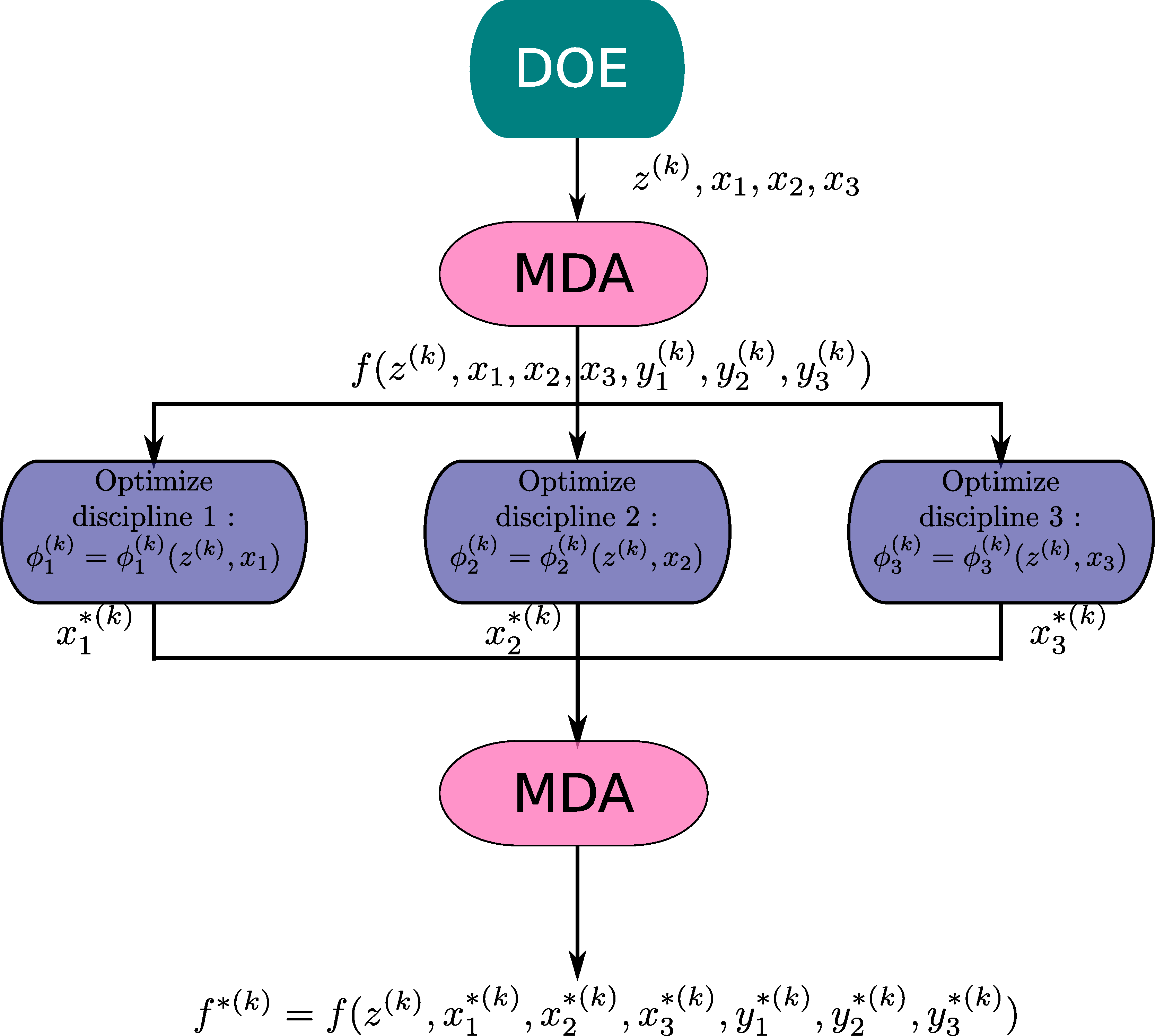
Description of the bilevel formulation process for trade-off

For Sobieski’s use case, the objective function is the range from the Breguet-Leduc equation:

\[Range = V. \underbrace{\left(\frac{L}{D}\right)}_{aerodynamics}.\underbrace{\frac {1}{SFC}}_{propulsion} \underbrace{\ln\left(\frac{W_T}{W_T-W_F}\right)}_{structure} \label{eqn:sobieski_range}\]

In this equation, each term is related to one of the three disciplines: aerodynamics, structure and propulsion. Therefore, in order to maximize the range, the disciplines should:

• maximize \((L/D)\) with respect to aerodynamics variables \(x_2\),

• minimize the Specific Fuel Consumption \(SFC\) with respect to propulsion variables \(x_3\),

• maximize \(\frac{W_T}{W_T-W_F}\) with respect to structure variables \(x_1\).

1. Define the disciplines

We first instantiate the MDODiscipline:

from gemseo.api import create_discipline

prop, aero, mission, struct = create_discipline(["SobieskiPropulsion", "SobieskiAerodynamics",
                                                 "SobieskiMission", "SobieskiStructure"])

2. Define the disciplinary design spaces

Then, for each disciplinary scenario, we

1. load the design space (function read_design_space()

2. keep only the design variables that are of interest for the scenario (function filter()):

from copy import deepcopy
from gemseo.api import read_design_space

input_file = join(dirname(__file__), "sobieski_design_space.txt")
design_space = read_design_space(input_file)
design_space_prop = deepcopy(design_space).filter("x_3")
design_space_aero = deepcopy(design_space).filter("x_2")
design_space_struct = deepcopy(design_space).filter("x_1")
design_space_mission = deepcopy(design_space).filter("x_shared")

3’. Define the disciplinary scenarios

The propulsion scenario minimizes the fuel specific consumption:

sc_prop = create_scenario(prop,
                          formulation="DisciplinaryOpt",
                          objective_name="y_34",
                          design_space=design_space_prop,
                          name="PropulsionScenario")

The aerodynamic scenario maximizes lift over drag:

sc_aero = create_scenario(aero,
                          formulation="DisciplinaryOpt",
                          objective_name="y_24",
                          design_space=design_space_aero,
                          name="AerodynamicsScenario",
                          maximize_objective=True)

The structure scenario maximizes \(log \frac{aircraft total weight}{aircraft total weight - fuel weight}\):

sc_struct = create_scenario(struct,
                            formulation="DisciplinaryOpt",
                            objective_name="y_11",
                            design_space=design_space_struct,
                            name="StructureScenario",
                            maximize_objective=True)

The range computation is added as a fourth discipline of the system scenario, which maximizes it:

sub_disciplines = [sc_prop, sc_aero, sc_struct]
sub_disciplines.append(mission)

for sub_sc in sub_disciplines[0:3]:
   sub_sc.default_inputs = {"max_iter": 20, "algo": "L-BFGS-B"}

Please also note that it is compulsory to set the default inputs of the first three disciplines, which are MDO scenarios. Thus, we have to set the optimization algorithm and the maximum number of iterations for each of them.

3’’. Define the main scenario

In a bi-level formulation, disciplinary optimizations are driven by the main (system-level) scenario which is a DOE (trade-off study), or an optimization process with respect to the system design variables (optimization problem).

system_scenario = create_scenario(sub_disciplines,
                                  formulation="BiLevel",
                                  objective_name="y_4",
                                  parallel_scenarios=False,
                                  # This is mandatory when doing
                                  # a DOE in parallel if we want
                                  # reproductible
                                  # results, dont reuse previous xopt
                                  reset_x0_before_opt=True,
                                  design_space=deepcopy(
                                      design_space).filter("x_shared"),
                                  maximize_objective=True,
                                  scenario_type="DOE")
# This is mandatory when doing
# a DOE in parallel if we want always exactly the same
# results, dont warm start mda1 to have exactely the same
# process whatever the execution order and process dispatch
system_scenario.formulation.mda1.warm_start = False
system_scenario.formulation.mda2.warm_start = False

4. Execute the trade-off study

Similarly to the disciplinary optimization scenarios, we create a dictionary of options (including all DOE settings) for the main scenario execution.

doe_options = {'n_samples': 30, 'algo': "lhs"}
system_scenario.execute(doe_options)

Comparison of trade-off results: bi-level versus MDF formulations

The aim of this section is to show the difference between MDF and bi-level trade-off studies presented in the previous section.

For MDF, the DOE requires a design space reduced to the sole system design variables, while the bi-level scenario involves disciplinary sub-optimization on the local design variables.

Some figures

As shown in the next figures, the bi-level scenario execution allows to reach a higher range than the MDF based scenario. This result highlights the interest of optimizing with respect to the local design variables when updating the system design variables.

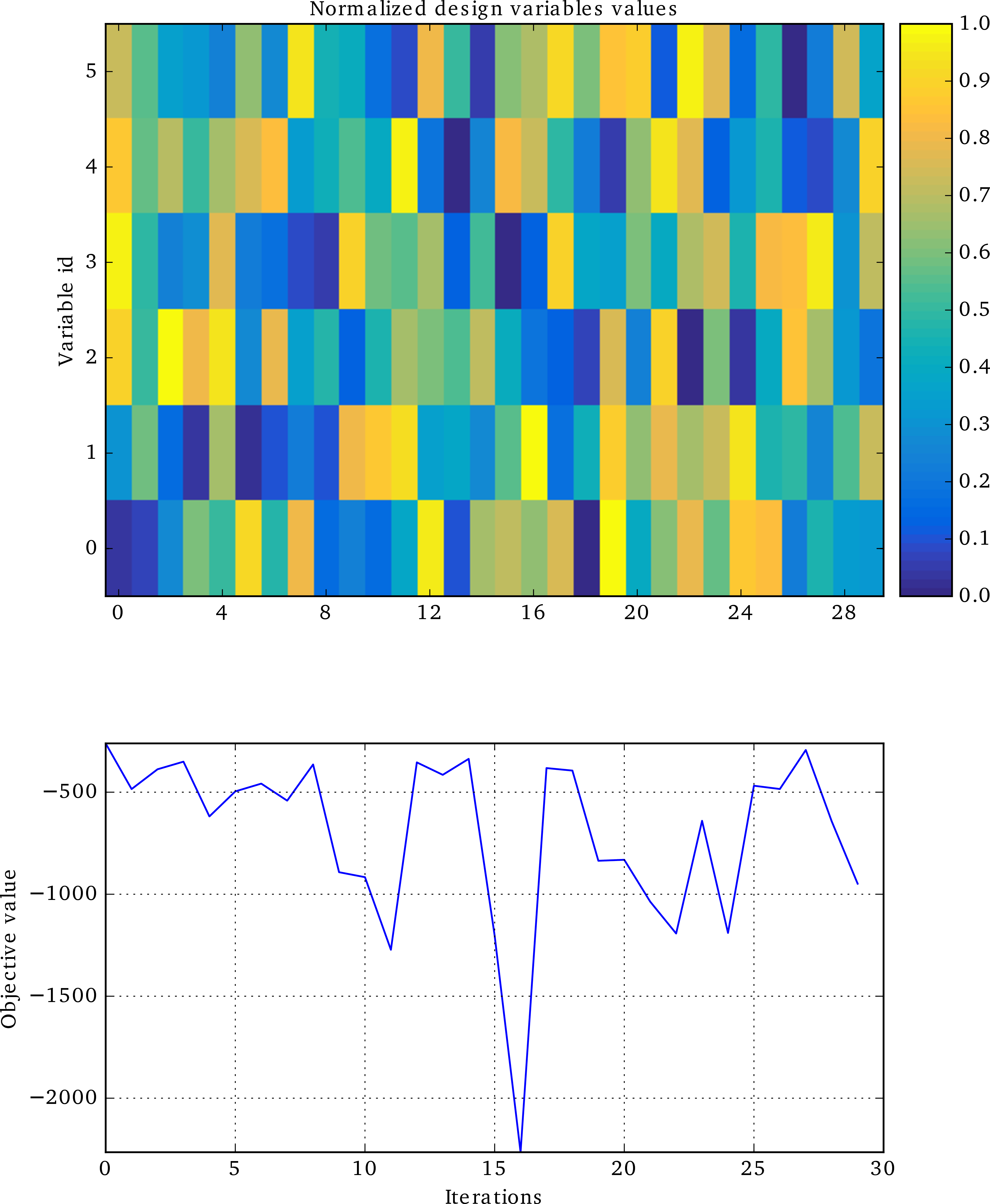
Bilevel DOE history

MDF DOE history

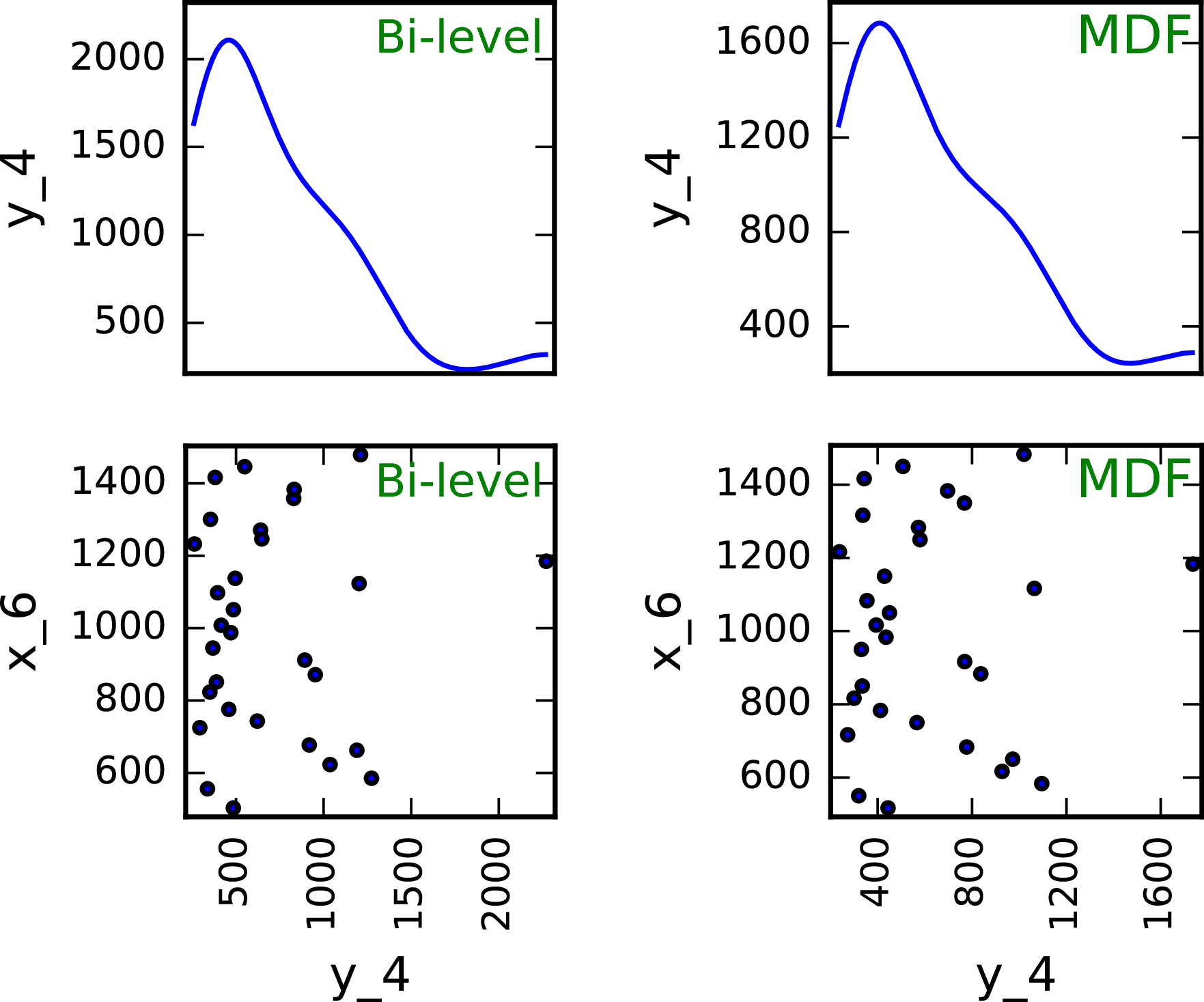
Comparison of and bi-level trade-off for a DOE of 30 samples

Remarks on the performance

One can note that with a of 30 samples, the best range found (about 1200 \(nm\)) is nowhere near the optimum found by the optimization process (a range of 3963 \(nm\) in less than 10 iterations). The last figure illustrates a trade-off study with 10,000 samples. Again, the best sample found (around 2600 \(nm\)) without any constraint consideration, is far from the optimal value. This example suggests that the sub-optimality trap is much more likely to happen with a trade-off study than with an optimization process.

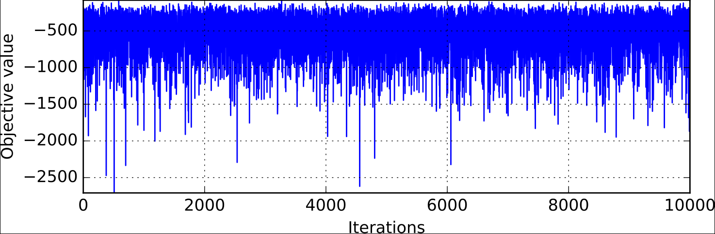
Objective function history for a DOE of 10,000 samples with MDF formulation