Solve a system of coupled ODEs

from __future__ import annotations

from itertools import starmap

from matplotlib import pyplot as plt
from numpy import linspace
from numpy.random import default_rng

from gemseo import create_discipline
from gemseo.core.chains.chain import MDOChain
from gemseo.disciplines.ode.ode_discipline import ODEDiscipline
from gemseo.mda.gauss_seidel import MDAGaussSeidel
from gemseo.problems.ode._springs import Mass
from gemseo.problems.ode._springs import create_chained_masses

This tutorial describes how to use the ODEDiscipline with coupled ODEs.

Problem description

Consider a set of point masses with masses \(m_1,\ m_2,...\ m_n\) connected by springs with stiffnesses \(k_1,\ k_2,...\ k_{n+1}\). The springs at each end of the system are connected to fixed points. We hereby study the response of the system to the displacement of one of the point masses.

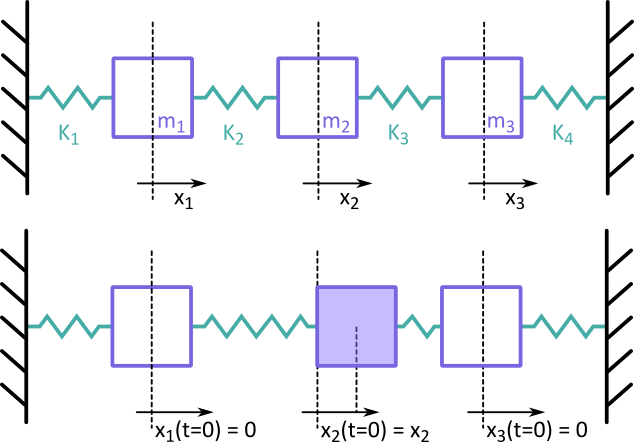
The motion of each point mass in this system is described by the following set of ordinary differential equations (ODEs):

\[\begin{split}\left\{ \begin{cases} \frac{dx_i}{dt} &= v_i \\ \frac{dv_i}{dt} &= - \frac{k_i + k_{i+1}}{m_i}x_i + \frac{k_i}{m_i}x_{i-1} + \frac{k_{i+1}}{m_i}x_{i+1} \end{cases} \right.\end{split}\]

where \(x_i\) is the position of the \(i\)-th point mass and \(v_i\) is its velocity.

These equations are coupled, since the forces applied to any given mass depend on the positions of its neighbors. In this tutorial, we will use the framework of the ODEDisciplines to solve this set of coupled equations.

Using an ODEDiscipline to solve the problem

Let's consider the problem described above in the case of two masses. First we describe the right-hand side (RHS) function of the equations of motion for each point mass.

stiffness_0 = 1
stiffness_1 = 1
stiffness_2 = 1
mass_0 = 1
mass_1 = 1
initial_position_0 = 1
initial_position_1 = 0
initial_velocity_0 = 0
initial_velocity_1 = 0

# Vector of times at which to solve the problem.
times = linspace(0, 1, 30)


def compute_mass_0_rhs(
    time=0,
    position_0=initial_position_0,
    velocity_0=initial_velocity_0,
    position_1=initial_position_1,
):
    """Compute the RHS of the ODE associated with the first point mass.

    Args:
        time: The time at which to evaluate the RHS.
        position_0: The position of the first point mass at this time.
        velocity_0: The velocity of the first point mass at this time.
        position_1: The position of the second point mass at this time.

    Returns:
        The first- and second-order derivatives of the position
        of the first point mass.
    """
    position_0_dot = velocity_0
    velocity_0_dot = (
        -(stiffness_0 + stiffness_1) * position_0 + stiffness_1 * position_1
    ) / mass_0
    return position_0_dot, velocity_0_dot


def compute_mass_1_rhs(
    time=0,
    position_1=initial_position_1,
    velocity_1=initial_velocity_1,
    position_0=initial_position_0,
):
    """Compute the RHS of the ODE associated with the secondpoint mass.

    Args:
        time: The time at which to evaluate the RHS.
        position_1: The position of the second point mass at this time.
        velocity_1: The velocity of the second point mass at this time.
        position_0: The position of the first point mass at this time.

    Returns:
        The first- and second-order derivatives of the position
        of the second point mass.
    """
    position_1_dot = velocity_1
    velocity_1_dot = (
        -(stiffness_1 + stiffness_2) * position_1 + stiffness_1 * position_0
    ) / mass_1
    return position_1_dot, velocity_1_dot

We can then create a list of ODEDiscipline objects

rhs_disciplines = [
    create_discipline("AutoPyDiscipline", py_func=compute_rhs)
    for compute_rhs in [compute_mass_0_rhs, compute_mass_1_rhs]
]
ode_disciplines = [
    ODEDiscipline(
        rhs_discipline,
        times,
        state_names=[f"position_{i}", f"velocity_{i}"],
        return_trajectories=True,
        rtol=1e-12,
        atol=1e-12,
    )
    for i, rhs_discipline in enumerate(rhs_disciplines)
]
for ode_discipline in ode_disciplines:
    ode_discipline.execute()

We apply an MDA with the Gauss-Seidel algorithm:

mda = MDAGaussSeidel(ode_disciplines)
local_data = mda.execute()

We can plot the residuals of this MDA.

mda.plot_residual_history()

<Figure size 640x480 with 1 Axes>

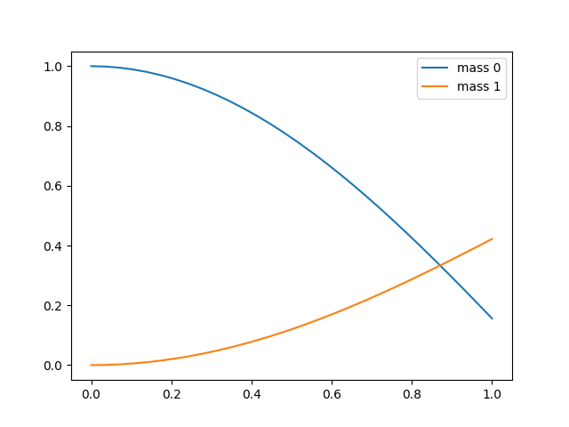
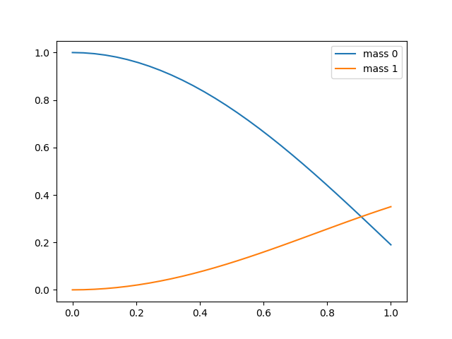
Plotting the solution

plt.plot(times, local_data["position_0_trajectory"], label="mass 0")
plt.plot(times, local_data["position_1_trajectory"], label="mass 1")
plt.legend()
plt.show()

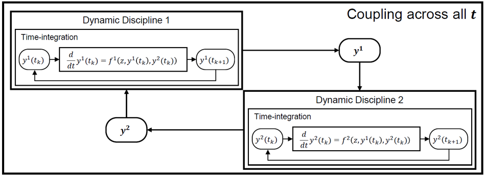
Another formulation

In the previous section, we considered the time-integration within each ODE discipline, then coupled the disciplines, as illustrated in the next figure.

Another possibility to tackle this problem is to define the couplings within a discipline, as illustrated in the next figure.

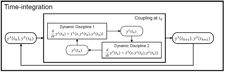
To do so, we can use the RHS disciplines we created earlier to define an MDOChain.

mda = MDOChain(rhs_disciplines)

We then define the ODE discipline that contains the couplings and execute it.

ode_discipline = ODEDiscipline(
    mda,
    times,
    state_names=["position_0", "velocity_0", "position_1", "velocity_1"],
    return_trajectories=True,
    rtol=1e-12,
    atol=1e-12,
)
local_data = ode_discipline.execute()

plt.plot(times, local_data["position_0_trajectory"], label="mass 0")
plt.plot(times, local_data["position_1_trajectory"], label="mass 1")
plt.legend()
plt.show()

Shortcut

The springs module provides a shortcut to access this problem. The user can define a list of masses, stiffnesses and initial positions, then create all the disciplines with a single call.

rng = default_rng(123)
masses = rng.random(3)
stiffnesses = rng.random(4)
positions = [1, 0, 0]
masses = list(starmap(Mass, zip(masses, stiffnesses[:-1], positions)))
chained_masses = create_chained_masses(stiffnesses[-1], *masses)
mda = MDOChain(chained_masses)
mda.execute()

{'position0': array([0.]), 'velocity0': array([0.]), 'time': array([0.]), 'position1_trajectory': array([0., 0., 0., 0., 0., 0., 0., 0., 0., 0., 0., 0., 0., 0., 0., 0., 0.,
       0., 0., 0., 0., 0., 0., 0., 0., 0., 0., 0., 0., 0.]), 'position1': array([0.]), 'velocity1': array([0.]), 'position2_trajectory': array([0., 0., 0., 0., 0., 0., 0., 0., 0., 0., 0., 0., 0., 0., 0., 0., 0.,
       0., 0., 0., 0., 0., 0., 0., 0., 0., 0., 0., 0., 0.]), 'position2': array([0.]), 'velocity2': array([0.]), 'position0_final': array([0.]), 'velocity0_final': array([0.]), 'position0_trajectory': array([0., 0., 0., 0., 0., 0., 0., 0., 0., 0., 0., 0., 0., 0., 0., 0., 0.,
       0., 0., 0., 0., 0., 0., 0., 0., 0., 0., 0., 0., 0.]), 'velocity0_trajectory': array([0., 0., 0., 0., 0., 0., 0., 0., 0., 0., 0., 0., 0., 0., 0., 0., 0.,
       0., 0., 0., 0., 0., 0., 0., 0., 0., 0., 0., 0., 0.]), 'termination_time': array([10.]), 'times': array([ 0.        ,  0.34482759,  0.68965517,  1.03448276,  1.37931034,
        1.72413793,  2.06896552,  2.4137931 ,  2.75862069,  3.10344828,
        3.44827586,  3.79310345,  4.13793103,  4.48275862,  4.82758621,
        5.17241379,  5.51724138,  5.86206897,  6.20689655,  6.55172414,
        6.89655172,  7.24137931,  7.5862069 ,  7.93103448,  8.27586207,
        8.62068966,  8.96551724,  9.31034483,  9.65517241, 10.        ]), 'position1_final': array([0.]), 'velocity1_final': array([0.]), 'velocity1_trajectory': array([0., 0., 0., 0., 0., 0., 0., 0., 0., 0., 0., 0., 0., 0., 0., 0., 0.,
       0., 0., 0., 0., 0., 0., 0., 0., 0., 0., 0., 0., 0.]), 'position2_final': array([0.]), 'velocity2_final': array([0.]), 'velocity2_trajectory': array([0., 0., 0., 0., 0., 0., 0., 0., 0., 0., 0., 0., 0., 0., 0., 0., 0.,
       0., 0., 0., 0., 0., 0., 0., 0., 0., 0., 0., 0., 0.])}