Solve a system of coupled ODEs

from __future__ import annotations

from typing import TYPE_CHECKING

from matplotlib import pyplot as plt
from numpy import array
from numpy import linspace
from scipy.interpolate import interp1d

from gemseo.core.chains.chain import MDOChain
from gemseo.core.discipline import Discipline
from gemseo.disciplines.auto_py import AutoPyDiscipline
from gemseo.disciplines.ode.ode_discipline import ODEDiscipline
from gemseo.mda.gauss_seidel import MDAGaussSeidel
from gemseo.problems.ode.springs.coupled_springs_generator import (
    CoupledSpringsGenerator,
)

if TYPE_CHECKING:
    from gemseo.typing import StrKeyMapping

This tutorial describes how to use the ODEDiscipline with coupled ODEs.

Problem description

Consider a set of point masses with masses \(m_1,\ m_2,...\ m_n\) connected by springs with stiffnesses \(k_1,\ k_2,...\ k_{n+1}\). The springs at each end of the system are connected to fixed points. We hereby study the response of the system to the displacement of one or multiple of the point masses.

The motion of each point mass in this system is described by the following set of ordinary differential equations (ODEs):

\[\begin{split}\begin{cases} \frac{dx_i}{dt} &= v_i \\ \frac{dv_i}{dt} &= - \frac{k_i + k_{i+1}}{m_i}x_i + \frac{k_i}{m_i}x_{i-1} + \frac{k_{i+1}}{m_i}x_{i+1} \end{cases}\end{split}\]

where \(x_i\) is the position of the \(i\)-th point mass and \(v_i\) is its velocity.

These equations are coupled, since the forces applied to any given mass depend on the positions of its neighbors. In this tutorial, we will use the framework of the ODEDisciplines to solve this set of coupled equations.

Using coupled instances of ODEDiscipline to solve the problem

Let us consider the problem described above in the case of two masses. First we describe the right-hand side (RHS) function of the equations of motion for each point mass.

ode_solver_name = "RK45"

stiffness_0 = 1
stiffness_1 = 1
stiffness_2 = 1
mass_0 = 1
mass_1 = 1

initial_position_0 = 1
initial_position_1 = 0
initial_velocity_0 = 0
initial_velocity_1 = 0

We define the times at which to discretize the trajectories.

times = linspace(0.0, 2.0, 30)

We define two disciplines to compute the RHS of the ODEs describing the dynamics of each mass.

class RHSMassDisciplineLeft(Discipline):
    def __init__(self, **kwargs) -> None:
        input_names = ("time", "position_0", "velocity_0", "position_1")
        output_names = ("position_0_dot", "velocity_0_dot")

        super().__init__(**kwargs)

        self.io.input_grammar.update_from_names(input_names)
        self.io.output_grammar.update_from_names(output_names)

        self.default_input_data = {
            "time": 0.0,
            "position_0": array([initial_position_0]),
            "velocity_0": array([initial_velocity_0]),
            "position_1": times * 0.0,
        }

        self.add_differentiated_inputs(["position_0", "velocity_0"])

    def _run(self, input_data: StrKeyMapping):
        time = self.io.data["time"]
        position_0 = self.io.data["position_0"]
        velocity_0 = self.io.data["velocity_0"]
        position_1_vec = self.io.data["position_1"]

        interp_function = interp1d(times, position_1_vec, assume_sorted=True)
        position_1 = interp_function(time)

        position_0_dot = velocity_0
        velocity_0_dot = (
            -(stiffness_0 + stiffness_1) * position_0 + stiffness_1 * position_1
        ) / mass_0

        self.local_data["position_0_dot"] = position_0_dot
        self.local_data["velocity_0_dot"] = velocity_0_dot


class RHSMassDisciplineRight(Discipline):
    def __init__(self, **kwargs) -> None:
        input_names = ("time", "position_1", "velocity_1", "position_0")
        output_names = ("position_1_dot", "velocity_1_dot")

        super().__init__(**kwargs)

        self.io.input_grammar.update_from_names(input_names)
        self.io.output_grammar.update_from_names(output_names)

        self.default_input_data = {
            "time": 0.0,
            "position_1": array([initial_position_1]),
            "velocity_1": array([initial_velocity_1]),
            "position_0": times * 0.0,
        }

        self.add_differentiated_inputs(["position_1", "velocity_1"])

    def _run(self, input_data: StrKeyMapping):
        time = self.io.data["time"]
        position_1 = self.io.data["position_1"]
        velocity_1 = self.io.data["velocity_1"]
        position_0_vec = self.io.data["position_0"]

        interp_function = interp1d(times, position_0_vec, assume_sorted=True)
        position_0 = interp_function(time)

        position_1_dot = velocity_1
        velocity_1_dot = (
            -(stiffness_0 + stiffness_1) * position_1 + stiffness_0 * position_0
        ) / mass_1

        self.local_data["position_1_dot"] = position_1_dot
        self.local_data["velocity_1_dot"] = velocity_1_dot

We can then create a list of ODEDiscipline objects

rhs_disciplines = [RHSMassDisciplineLeft(), RHSMassDisciplineRight()]

ode_disciplines = [
    ODEDiscipline(
        rhs_discipline=rhs_discipline,
        times=times,
        state_names=(f"position_{i}", f"velocity_{i}"),
        time_name="time",
        return_trajectories=True,
        ode_solver_name=ode_solver_name,
        rtol=1e-6,
        atol=1e-6,
    )
    for i, rhs_discipline in enumerate(rhs_disciplines)
]
for ode_discipline in ode_disciplines:
    ode_discipline.execute()

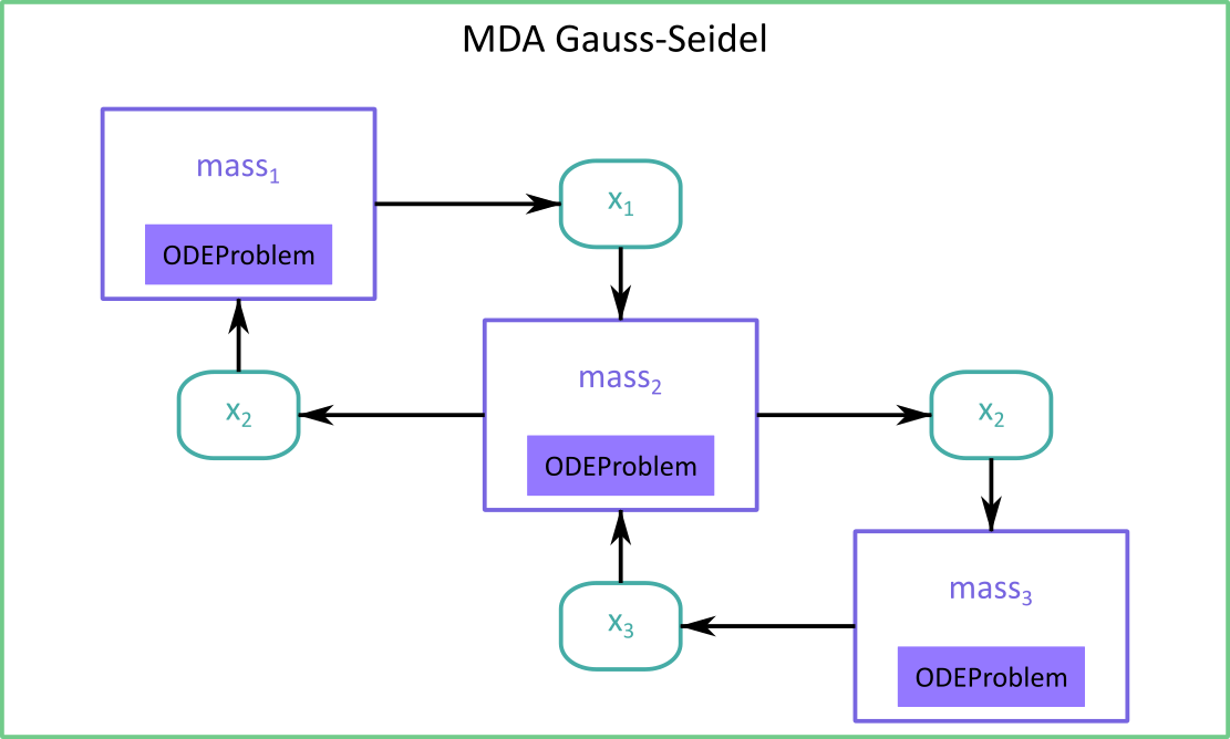
We apply an MDA with the Gauss-Seidel algorithm:

mda = MDAGaussSeidel(ode_disciplines)
local_data = mda.execute()

WARNING - 16:21:55: Two disciplines, among which ODEDiscipline, compute the same outputs: {'times', 'termination_time'}
WARNING - 16:21:55: Self coupling variables in discipline ODEDiscipline are: ['times'].
WARNING - 16:21:55: Self coupling variables in discipline ODEDiscipline are: ['times'].
WARNING - 16:21:55: The following disciplines contain self-couplings and strong couplings: ['ODEDiscipline', 'ODEDiscipline']. This is not a problem as long as their self-coupling variables are not strongly coupled to another discipline.
WARNING - 16:21:55: The following outputs are defined multiple times: ['termination_time', 'times'].

The coupling structure between the instances of ODEDiscipline can be represented by the following picture.

We can plot the residuals of this MDA.

mda.plot_residual_history()

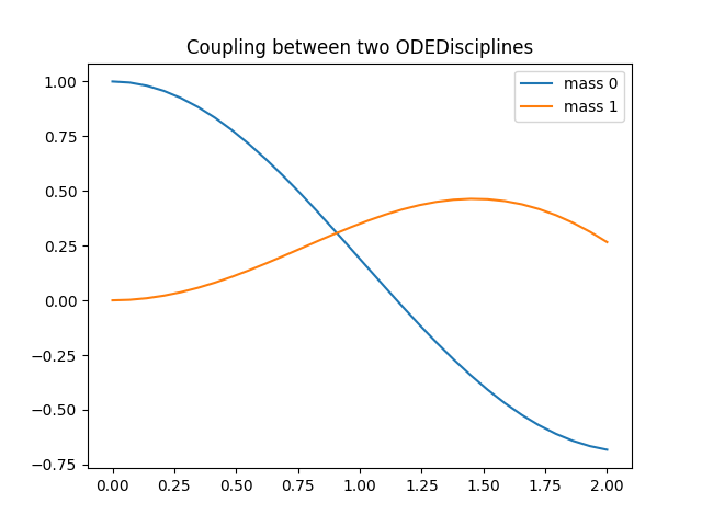
plt.plot(times, local_data["position_0"], label="mass 0")
plt.plot(times, local_data["position_1"], label="mass 1")
plt.title("Coupling between two ODEDisciplines")
plt.legend()
plt.show()

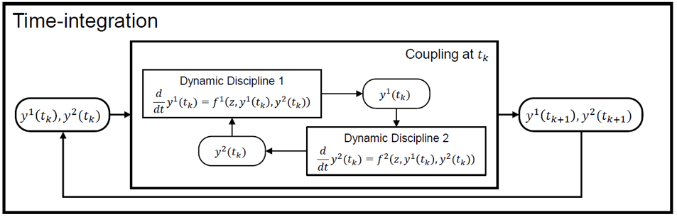
Using a single ODEDiscipline with coupled dynamics

In the previous section, we considered the integration in time within each ODE discipline, then coupled the disciplines, as illustrated in the next figure. Another possibility to tackle this problem is to define the couplings within a discipline, as illustrated in the next figure.

def compute_mass_0_rhs(
    time=0,
    position_0=initial_position_0,
    velocity_0=initial_velocity_0,
    position_1=initial_position_1,
):
    """Compute the RHS of the ODE associated with the first point mass.

    Args:
        time: The time at which to evaluate the RHS.
        position_0: The position of the first point mass at this time.
        velocity_0: The velocity of the first point mass at this time.
        position_1: The position of the second point mass at this time.

    Returns:
        The first- and second-order derivatives of the position
        of the first point mass.
    """

    position_0_dot = velocity_0
    velocity_0_dot = (
        -(stiffness_0 + stiffness_1) * position_0 + stiffness_1 * position_1
    ) / mass_0
    return position_0_dot, velocity_0_dot


def compute_mass_1_rhs(
    time=0,
    position_1=initial_position_1,
    velocity_1=initial_velocity_1,
    position_0=initial_position_0,
):
    """Compute the RHS of the ODE associated with the second point mass.

    Args:
        time: The time at which to evaluate the RHS.
        position_1: The position of the second point mass at this time.
        velocity_1: The velocity of the second point mass at this time.
        position_0: The position of the first point mass at this time.

    Returns:
        The first- and second-order derivatives of the position
        of the second point mass.
    """
    position_1_dot = velocity_1
    velocity_1_dot = (
        -(stiffness_1 + stiffness_2) * position_1 + stiffness_1 * position_0
    ) / mass_1
    return position_1_dot, velocity_1_dot

To do so, we can use the RHS disciplines we created earlier to define an MDOChain.

rhs_disciplines = [
    AutoPyDiscipline(py_func=compute_rhs)
    for compute_rhs in [compute_mass_0_rhs, compute_mass_1_rhs]
]

rhs_disciplines[0].add_differentiated_inputs(["time", "position_0", "velocity_0"])
rhs_disciplines[1].add_differentiated_inputs(["time", "position_1", "velocity_1"])

mda = MDOChain(rhs_disciplines)

We then define the ODE discipline that contains the couplings and execute it.

ode_discipline = ODEDiscipline(
    rhs_discipline=mda,
    state_names={
        "position_0": "position_0_dot",
        "velocity_0": "velocity_0_dot",
        "position_1": "position_1_dot",
        "velocity_1": "velocity_1_dot",
    },
    return_trajectories=True,
    times=times,
    ode_solver_name=ode_solver_name,
    rtol=1e-12,
    atol=1e-12,
)
local_data = ode_discipline.execute()


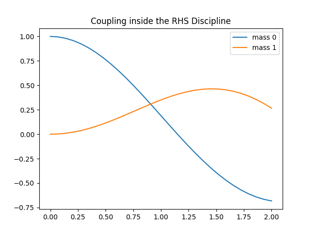
plt.plot(times, local_data["position_0"], label="mass 0")
plt.plot(times, local_data["position_1"], label="mass 1")
plt.title("Coupling inside the RHS Discipline")
plt.legend()
plt.show()

Shortcut

The springs module provides shortcuts to access this problem. The user can define a list of masses, stiffnesses and initial positions, then create all the disciplines with a single call using the class CoupledSpringsGenerator.

masses = [1, 2, 1]
stiffnesses = [1, 1, 1, 1]
positions = [1, 0, 0]

springs_and_masses = CoupledSpringsGenerator(
    masses=masses, stiffnesses=stiffnesses, times=times
)

The method 'coupled_ode_disciplines' of CoupledSpringsGenerator creates a list of ODEDiscipline. Each discipline is used to compute the movement of a single mass. The disciplines can be coupled with one another by an MDA.

disciplines = springs_and_masses.create_coupled_ode_disciplines(
    atol=1e-8, ode_solver_name=ode_solver_name
)
mda_shortcut = MDAGaussSeidel(disciplines)

mda_result = mda_shortcut.execute({
    "initial_position_0": array([positions[0]]),
    "initial_position_1": array([positions[1]]),
    "initial_position_2": array([positions[2]]),
})

WARNING - 16:21:56: Two disciplines, among which SpringODEDiscipline, compute the same outputs: {'times', 'termination_time'}
WARNING - 16:21:56: Self coupling variables in discipline SpringODEDiscipline are: ['times'].
WARNING - 16:21:56: Self coupling variables in discipline SpringODEDiscipline are: ['times'].
WARNING - 16:21:56: Self coupling variables in discipline SpringODEDiscipline are: ['times'].
WARNING - 16:21:56: The following disciplines contain self-couplings and strong couplings: ['SpringODEDiscipline', 'SpringODEDiscipline', 'SpringODEDiscipline']. This is not a problem as long as their self-coupling variables are not strongly coupled to another discipline.
WARNING - 16:21:56: The following outputs are defined multiple times: ['termination_time', 'termination_time', 'times', 'times'].

The method CoupledSpringsGenerator.discipline_with_coupled_dynamic() of CoupledSpringsGenerator returns a single instance of ODEDiscipline, whose dynamic is defined by an MDA on the dynamics of all masses in the system.

ode_discipline_shortcut = springs_and_masses.create_discipline_with_coupled_dynamics(
    ode_solver_name=ode_solver_name
)
ode_result = ode_discipline_shortcut.execute({
    "initial_position_0": array([positions[0]]),
    "initial_position_1": array([positions[1]]),
    "initial_position_2": array([positions[2]]),
})

We can plot and compare the results.

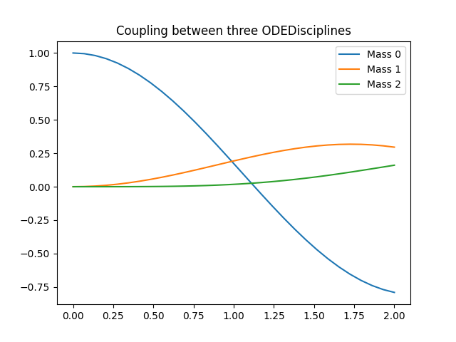
The trajectories of three masses computed by coupling three instances of ODEDiscipline.

plt.plot(times, mda_result["position_0"], label="Mass 0")
plt.plot(times, mda_result["position_1"], label="Mass 1")
plt.plot(times, mda_result["position_2"], label="Mass 2")
plt.title("Coupling between three ODEDisciplines")
plt.legend()
plt.show()

The trajectories of three masses computed by one instance of ODEDiscipline with a dynamic defined by three coupled disciplines.

plt.plot(times, ode_result["position_0"], label="Mass 0")
plt.plot(times, ode_result["position_1"], label="Mass 1")
plt.plot(times, ode_result["position_2"], label="Mass 2")
plt.title("Triple coupling inside the RHS Discipline")
plt.legend()
plt.show()

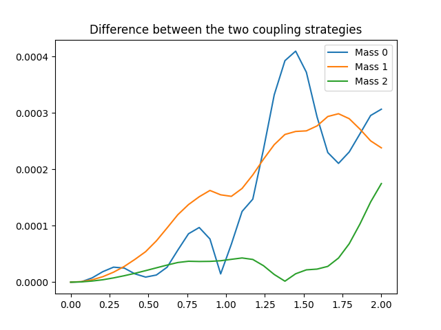
Absolute value of the difference between the two methods.

error_position_0 = abs(mda_result["position_0"] - ode_result["position_0"])
error_position_1 = abs(mda_result["position_1"] - ode_result["position_1"])
error_position_2 = abs(mda_result["position_2"] - ode_result["position_2"])

plt.plot(times, error_position_0, label="Mass 0")
plt.plot(times, error_position_1, label="Mass 1")
plt.plot(times, error_position_2, label="Mass 2")
plt.title("Difference between the two coupling strategies")
plt.legend()
plt.show()