Note
Go to the end to download the full example code.
How to solve an optimization problem#
Although the GEMSEO library is dedicated to the MDO, it can also be used for mono-disciplinary optimization problems. This example presents some analytical test cases.
Imports#
from __future__ import annotations

import numpy as np
from scipy import optimize

from gemseo import create_design_space
from gemseo import create_discipline
from gemseo import create_scenario
from gemseo import execute_post
from gemseo import get_available_opt_algorithms
Optimization based on a design of experiments#
Let \((P)\) be a simple optimization problem:
In this section, we will see how to use GEMSEO to solve this problem \((P)\) by means of a Design Of Experiments (DOE)
Define the objective function#
Firstly, by means of the create_discipline() high-level function,
we create a Discipline of AutoPyDiscipline type
from a Python function.
def f(x1=0.0, x2=0.0):
    y = x1 + x2
    return y


discipline = create_discipline("AutoPyDiscipline", py_func=f)
Now, we want to minimize this Discipline over a design of experiments (DOE).
Define the design space#
For that, by means of the create_design_space() API function,
we define the DesignSpace \([-5, 5]\times[-5, 5]\)
by using its add_variable() method.
design_space = create_design_space()
design_space.add_variable("x1", 1, lower_bound=-5, upper_bound=5, type_="integer")
design_space.add_variable("x2", 1, lower_bound=-5, upper_bound=5, type_="integer")
Define the DOE scenario#
Then, by means of the create_scenario() high-level function,
we define a DOEScenario from the Discipline
and the DesignSpace defined above:
scenario = create_scenario(
    discipline,
    "y",
    design_space,
    formulation_name="DisciplinaryOpt",
    scenario_type="DOE",
)
Execute the DOE scenario#
Lastly, we solve the OptimizationProblem included in the
DOEScenario defined above by minimizing the objective function over a
design of experiments included in the DesignSpace.
Precisely, we choose a
full factorial design
of size \(11^2\):
scenario.execute(algo_name="PYDOE_FULLFACT", n_samples=11**2)
INFO - 16:25:01: *** Start DOEScenario execution ***
INFO - 16:25:01: DOEScenario
INFO - 16:25:01:    Disciplines: f
INFO - 16:25:01:    MDO formulation: DisciplinaryOpt
INFO - 16:25:01: Optimization problem:
INFO - 16:25:01:    minimize y(x1, x2)
INFO - 16:25:01:    with respect to x1, x2
INFO - 16:25:01:    over the design space:
INFO - 16:25:01:       +------+-------------+-------+-------------+---------+
INFO - 16:25:01:       | Name | Lower bound | Value | Upper bound | Type    |
INFO - 16:25:01:       +------+-------------+-------+-------------+---------+
INFO - 16:25:01:       | x1   |      -5     |  None |      5      | integer |
INFO - 16:25:01:       | x2   |      -5     |  None |      5      | integer |
INFO - 16:25:01:       +------+-------------+-------+-------------+---------+
INFO - 16:25:01: Solving optimization problem with algorithm PYDOE_FULLFACT:
INFO - 16:25:01:      1%|          | 1/121 [00:00<00:00, 566.87 it/sec, feas=True, obj=-10]
INFO - 16:25:01:      2%|▏         | 2/121 [00:00<00:00, 970.57 it/sec, feas=True, obj=-9]
INFO - 16:25:01:      2%|▏         | 3/121 [00:00<00:00, 1304.47 it/sec, feas=True, obj=-8]
INFO - 16:25:01:      3%|▎         | 4/121 [00:00<00:00, 1585.15 it/sec, feas=True, obj=-7]
INFO - 16:25:01:      4%|▍         | 5/121 [00:00<00:00, 1807.89 it/sec, feas=True, obj=-6]
INFO - 16:25:01:      5%|▍         | 6/121 [00:00<00:00, 2013.91 it/sec, feas=True, obj=-5]
INFO - 16:25:01:      6%|▌         | 7/121 [00:00<00:00, 2189.91 it/sec, feas=True, obj=-4]
INFO - 16:25:01:      7%|▋         | 8/121 [00:00<00:00, 2346.96 it/sec, feas=True, obj=-3]
INFO - 16:25:01:      7%|▋         | 9/121 [00:00<00:00, 2469.66 it/sec, feas=True, obj=-2]
INFO - 16:25:01:      8%|▊         | 10/121 [00:00<00:00, 2591.00 it/sec, feas=True, obj=-1]
INFO - 16:25:01:      9%|▉         | 11/121 [00:00<00:00, 2703.62 it/sec, feas=True, obj=0]
INFO - 16:25:01:     10%|▉         | 12/121 [00:00<00:00, 2810.10 it/sec, feas=True, obj=-9]
INFO - 16:25:01:     11%|█         | 13/121 [00:00<00:00, 2907.90 it/sec, feas=True, obj=-8]
INFO - 16:25:01:     12%|█▏        | 14/121 [00:00<00:00, 2987.24 it/sec, feas=True, obj=-7]
INFO - 16:25:01:     12%|█▏        | 15/121 [00:00<00:00, 3068.70 it/sec, feas=True, obj=-6]
INFO - 16:25:01:     13%|█▎        | 16/121 [00:00<00:00, 3146.96 it/sec, feas=True, obj=-5]
INFO - 16:25:01:     14%|█▍        | 17/121 [00:00<00:00, 3213.74 it/sec, feas=True, obj=-4]
INFO - 16:25:01:     15%|█▍        | 18/121 [00:00<00:00, 3281.93 it/sec, feas=True, obj=-3]
INFO - 16:25:01:     16%|█▌        | 19/121 [00:00<00:00, 3328.12 it/sec, feas=True, obj=-2]
INFO - 16:25:01:     17%|█▋        | 20/121 [00:00<00:00, 3377.46 it/sec, feas=True, obj=-1]
INFO - 16:25:01:     17%|█▋        | 21/121 [00:00<00:00, 3426.05 it/sec, feas=True, obj=0]
INFO - 16:25:01:     18%|█▊        | 22/121 [00:00<00:00, 3474.07 it/sec, feas=True, obj=1]
INFO - 16:25:01:     19%|█▉        | 23/121 [00:00<00:00, 3515.25 it/sec, feas=True, obj=-8]
INFO - 16:25:01:     20%|█▉        | 24/121 [00:00<00:00, 3541.74 it/sec, feas=True, obj=-7]
INFO - 16:25:01:     21%|██        | 25/121 [00:00<00:00, 3581.08 it/sec, feas=True, obj=-6]
INFO - 16:25:01:     21%|██▏       | 26/121 [00:00<00:00, 3616.86 it/sec, feas=True, obj=-5]
INFO - 16:25:01:     22%|██▏       | 27/121 [00:00<00:00, 3654.05 it/sec, feas=True, obj=-4]
INFO - 16:25:01:     23%|██▎       | 28/121 [00:00<00:00, 3682.56 it/sec, feas=True, obj=-3]
INFO - 16:25:01:     24%|██▍       | 29/121 [00:00<00:00, 3714.27 it/sec, feas=True, obj=-2]
INFO - 16:25:01:     25%|██▍       | 30/121 [00:00<00:00, 3742.58 it/sec, feas=True, obj=-1]
INFO - 16:25:01:     26%|██▌       | 31/121 [00:00<00:00, 3769.67 it/sec, feas=True, obj=0]
INFO - 16:25:01:     26%|██▋       | 32/121 [00:00<00:00, 3794.03 it/sec, feas=True, obj=1]
INFO - 16:25:01:     27%|██▋       | 33/121 [00:00<00:00, 3808.18 it/sec, feas=True, obj=2]
INFO - 16:25:01:     28%|██▊       | 34/121 [00:00<00:00, 3827.23 it/sec, feas=True, obj=-7]
INFO - 16:25:01:     29%|██▉       | 35/121 [00:00<00:00, 3844.96 it/sec, feas=True, obj=-6]
INFO - 16:25:01:     30%|██▉       | 36/121 [00:00<00:00, 3858.11 it/sec, feas=True, obj=-5]
INFO - 16:25:01:     31%|███       | 37/121 [00:00<00:00, 3876.05 it/sec, feas=True, obj=-4]
INFO - 16:25:01:     31%|███▏      | 38/121 [00:00<00:00, 3886.08 it/sec, feas=True, obj=-3]
INFO - 16:25:01:     32%|███▏      | 39/121 [00:00<00:00, 3903.91 it/sec, feas=True, obj=-2]
INFO - 16:25:01:     33%|███▎      | 40/121 [00:00<00:00, 3920.92 it/sec, feas=True, obj=-1]
INFO - 16:25:01:     34%|███▍      | 41/121 [00:00<00:00, 3937.86 it/sec, feas=True, obj=0]
INFO - 16:25:01:     35%|███▍      | 42/121 [00:00<00:00, 3945.64 it/sec, feas=True, obj=1]
INFO - 16:25:01:     36%|███▌      | 43/121 [00:00<00:00, 3958.63 it/sec, feas=True, obj=2]
INFO - 16:25:01:     36%|███▋      | 44/121 [00:00<00:00, 3973.67 it/sec, feas=True, obj=3]
INFO - 16:25:01:     37%|███▋      | 45/121 [00:00<00:00, 3988.58 it/sec, feas=True, obj=-6]
INFO - 16:25:01:     38%|███▊      | 46/121 [00:00<00:00, 4003.36 it/sec, feas=True, obj=-5]
INFO - 16:25:01:     39%|███▉      | 47/121 [00:00<00:00, 4009.36 it/sec, feas=True, obj=-4]
INFO - 16:25:01:     40%|███▉      | 48/121 [00:00<00:00, 3985.88 it/sec, feas=True, obj=-3]
INFO - 16:25:01:     40%|████      | 49/121 [00:00<00:00, 3994.26 it/sec, feas=True, obj=-2]
INFO - 16:25:01:     41%|████▏     | 50/121 [00:00<00:00, 4005.10 it/sec, feas=True, obj=-1]
INFO - 16:25:01:     42%|████▏     | 51/121 [00:00<00:00, 4009.70 it/sec, feas=True, obj=0]
INFO - 16:25:01:     43%|████▎     | 52/121 [00:00<00:00, 4022.35 it/sec, feas=True, obj=1]
INFO - 16:25:01:     44%|████▍     | 53/121 [00:00<00:00, 4030.50 it/sec, feas=True, obj=2]
INFO - 16:25:01:     45%|████▍     | 54/121 [00:00<00:00, 4042.34 it/sec, feas=True, obj=3]
INFO - 16:25:01:     45%|████▌     | 55/121 [00:00<00:00, 4050.69 it/sec, feas=True, obj=4]
INFO - 16:25:01:     46%|████▋     | 56/121 [00:00<00:00, 4062.35 it/sec, feas=True, obj=-5]
INFO - 16:25:01:     47%|████▋     | 57/121 [00:00<00:00, 4075.68 it/sec, feas=True, obj=-4]
INFO - 16:25:01:     48%|████▊     | 58/121 [00:00<00:00, 4089.73 it/sec, feas=True, obj=-3]
INFO - 16:25:01:     49%|████▉     | 59/121 [00:00<00:00, 4104.49 it/sec, feas=True, obj=-2]
INFO - 16:25:01:     50%|████▉     | 60/121 [00:00<00:00, 4112.73 it/sec, feas=True, obj=-1]
INFO - 16:25:01:     50%|█████     | 61/121 [00:00<00:00, 4122.33 it/sec, feas=True, obj=0]
INFO - 16:25:01:     51%|█████     | 62/121 [00:00<00:00, 4134.68 it/sec, feas=True, obj=1]
INFO - 16:25:01:     52%|█████▏    | 63/121 [00:00<00:00, 4147.04 it/sec, feas=True, obj=2]
INFO - 16:25:01:     53%|█████▎    | 64/121 [00:00<00:00, 4158.95 it/sec, feas=True, obj=3]
INFO - 16:25:01:     54%|█████▎    | 65/121 [00:00<00:00, 4166.10 it/sec, feas=True, obj=4]
INFO - 16:25:01:     55%|█████▍    | 66/121 [00:00<00:00, 4175.01 it/sec, feas=True, obj=5]
INFO - 16:25:01:     55%|█████▌    | 67/121 [00:00<00:00, 4186.37 it/sec, feas=True, obj=-4]
INFO - 16:25:01:     56%|█████▌    | 68/121 [00:00<00:00, 4197.21 it/sec, feas=True, obj=-3]
INFO - 16:25:01:     57%|█████▋    | 69/121 [00:00<00:00, 4207.66 it/sec, feas=True, obj=-2]
INFO - 16:25:01:     58%|█████▊    | 70/121 [00:00<00:00, 4212.54 it/sec, feas=True, obj=-1]
INFO - 16:25:01:     59%|█████▊    | 71/121 [00:00<00:00, 4221.18 it/sec, feas=True, obj=0]
INFO - 16:25:01:     60%|█████▉    | 72/121 [00:00<00:00, 4230.26 it/sec, feas=True, obj=1]
INFO - 16:25:01:     60%|██████    | 73/121 [00:00<00:00, 4237.78 it/sec, feas=True, obj=2]
INFO - 16:25:01:     61%|██████    | 74/121 [00:00<00:00, 4248.33 it/sec, feas=True, obj=3]
INFO - 16:25:01:     62%|██████▏   | 75/121 [00:00<00:00, 4253.92 it/sec, feas=True, obj=4]
INFO - 16:25:01:     63%|██████▎   | 76/121 [00:00<00:00, 4261.93 it/sec, feas=True, obj=5]
INFO - 16:25:01:     64%|██████▎   | 77/121 [00:00<00:00, 4271.64 it/sec, feas=True, obj=6]
INFO - 16:25:01:     64%|██████▍   | 78/121 [00:00<00:00, 4280.85 it/sec, feas=True, obj=-3]
INFO - 16:25:01:     65%|██████▌   | 79/121 [00:00<00:00, 4290.43 it/sec, feas=True, obj=-2]
INFO - 16:25:01:     66%|██████▌   | 80/121 [00:00<00:00, 4294.42 it/sec, feas=True, obj=-1]
INFO - 16:25:01:     67%|██████▋   | 81/121 [00:00<00:00, 4301.58 it/sec, feas=True, obj=0]
INFO - 16:25:01:     68%|██████▊   | 82/121 [00:00<00:00, 4309.61 it/sec, feas=True, obj=1]
INFO - 16:25:01:     69%|██████▊   | 83/121 [00:00<00:00, 4318.93 it/sec, feas=True, obj=2]
INFO - 16:25:01:     69%|██████▉   | 84/121 [00:00<00:00, 4328.27 it/sec, feas=True, obj=3]
INFO - 16:25:01:     70%|███████   | 85/121 [00:00<00:00, 4333.06 it/sec, feas=True, obj=4]
INFO - 16:25:01:     71%|███████   | 86/121 [00:00<00:00, 4339.89 it/sec, feas=True, obj=5]
INFO - 16:25:01:     72%|███████▏  | 87/121 [00:00<00:00, 4348.09 it/sec, feas=True, obj=6]
INFO - 16:25:01:     73%|███████▎  | 88/121 [00:00<00:00, 4356.43 it/sec, feas=True, obj=7]
INFO - 16:25:01:     74%|███████▎  | 89/121 [00:00<00:00, 4364.01 it/sec, feas=True, obj=-2]
INFO - 16:25:01:     74%|███████▍  | 90/121 [00:00<00:00, 4366.59 it/sec, feas=True, obj=-1]
INFO - 16:25:01:     75%|███████▌  | 91/121 [00:00<00:00, 4373.02 it/sec, feas=True, obj=0]
INFO - 16:25:01:     76%|███████▌  | 92/121 [00:00<00:00, 4380.87 it/sec, feas=True, obj=1]
INFO - 16:25:01:     77%|███████▋  | 93/121 [00:00<00:00, 4385.72 it/sec, feas=True, obj=2]
INFO - 16:25:01:     78%|███████▊  | 94/121 [00:00<00:00, 4392.68 it/sec, feas=True, obj=3]
INFO - 16:25:01:     79%|███████▊  | 95/121 [00:00<00:00, 4395.72 it/sec, feas=True, obj=4]
INFO - 16:25:01:     79%|███████▉  | 96/121 [00:00<00:00, 4401.50 it/sec, feas=True, obj=5]
INFO - 16:25:01:     80%|████████  | 97/121 [00:00<00:00, 4407.31 it/sec, feas=True, obj=6]
INFO - 16:25:01:     81%|████████  | 98/121 [00:00<00:00, 4414.11 it/sec, feas=True, obj=7]
INFO - 16:25:01:     82%|████████▏ | 99/121 [00:00<00:00, 4421.31 it/sec, feas=True, obj=8]
INFO - 16:25:01:     83%|████████▎ | 100/121 [00:00<00:00, 4422.65 it/sec, feas=True, obj=-1]
INFO - 16:25:01:     83%|████████▎ | 101/121 [00:00<00:00, 4426.87 it/sec, feas=True, obj=0]
INFO - 16:25:01:     84%|████████▍ | 102/121 [00:00<00:00, 4433.04 it/sec, feas=True, obj=1]
INFO - 16:25:01:     85%|████████▌ | 103/121 [00:00<00:00, 4439.01 it/sec, feas=True, obj=2]
INFO - 16:25:01:     86%|████████▌ | 104/121 [00:00<00:00, 4445.07 it/sec, feas=True, obj=3]
INFO - 16:25:01:     87%|████████▋ | 105/121 [00:00<00:00, 4447.52 it/sec, feas=True, obj=4]
INFO - 16:25:01:     88%|████████▊ | 106/121 [00:00<00:00, 4452.69 it/sec, feas=True, obj=5]
INFO - 16:25:01:     88%|████████▊ | 107/121 [00:00<00:00, 4458.88 it/sec, feas=True, obj=6]
INFO - 16:25:01:     89%|████████▉ | 108/121 [00:00<00:00, 4464.75 it/sec, feas=True, obj=7]
INFO - 16:25:01:     90%|█████████ | 109/121 [00:00<00:00, 4470.05 it/sec, feas=True, obj=8]
INFO - 16:25:01:     91%|█████████ | 110/121 [00:00<00:00, 4472.23 it/sec, feas=True, obj=9]
INFO - 16:25:01:     92%|█████████▏| 111/121 [00:00<00:00, 4476.35 it/sec, feas=True, obj=0]
INFO - 16:25:01:     93%|█████████▎| 112/121 [00:00<00:00, 4481.22 it/sec, feas=True, obj=1]
INFO - 16:25:01:     93%|█████████▎| 113/121 [00:00<00:00, 4484.15 it/sec, feas=True, obj=2]
INFO - 16:25:01:     94%|█████████▍| 114/121 [00:00<00:00, 4488.58 it/sec, feas=True, obj=3]
INFO - 16:25:01:     95%|█████████▌| 115/121 [00:00<00:00, 4490.02 it/sec, feas=True, obj=4]
INFO - 16:25:01:     96%|█████████▌| 116/121 [00:00<00:00, 4493.84 it/sec, feas=True, obj=5]
INFO - 16:25:01:     97%|█████████▋| 117/121 [00:00<00:00, 4498.80 it/sec, feas=True, obj=6]
INFO - 16:25:01:     98%|█████████▊| 118/121 [00:00<00:00, 4503.40 it/sec, feas=True, obj=7]
INFO - 16:25:01:     98%|█████████▊| 119/121 [00:00<00:00, 4506.91 it/sec, feas=True, obj=8]
INFO - 16:25:01:     99%|█████████▉| 120/121 [00:00<00:00, 4507.94 it/sec, feas=True, obj=9]
INFO - 16:25:01:    100%|██████████| 121/121 [00:00<00:00, 4471.30 it/sec, feas=True, obj=10]
INFO - 16:25:01: Optimization result:
INFO - 16:25:01:    Optimizer info:
INFO - 16:25:01:       Status: None
INFO - 16:25:01:       Message: None
INFO - 16:25:01:    Solution:
INFO - 16:25:01:       Objective: -10.0
INFO - 16:25:01:       Design space:
INFO - 16:25:01:          +------+-------------+-------+-------------+---------+
INFO - 16:25:01:          | Name | Lower bound | Value | Upper bound | Type    |
INFO - 16:25:01:          +------+-------------+-------+-------------+---------+
INFO - 16:25:01:          | x1   |      -5     |   -5  |      5      | integer |
INFO - 16:25:01:          | x2   |      -5     |   -5  |      5      | integer |
INFO - 16:25:01:          +------+-------------+-------+-------------+---------+
INFO - 16:25:01: *** End DOEScenario execution ***
The optimum results can be found in the execution log. It is also possible to
extract them from the BaseScenario.optimization_result.
optimization_result = scenario.optimization_result
print(
    f"The solution of P is (x*,f(x*)) = ({optimization_result.x_opt}, {optimization_result.f_opt})"
)
The solution of P is (x*,f(x*)) = ([-5. -5.], -10.0)
Optimization based on a quasi-Newton method by means of the SciPy library#
Let \((P)\) be a simple optimization problem:
In this section, we will see how to use GEMSEO to solve this problem \((P)\) by means of an optimizer directly used from the SciPy library.
Define the objective function#
Firstly, we create the objective function and its gradient as standard Python functions:
def g(x=0):
    y = np.sin(x) - np.exp(x)
    return y


def dgdx(x=0):
    y = np.cos(x) - np.exp(x)
    return y
Minimize the objective function#
Now, we can minimize this Python function over its design space by means of
the L-BFGS-B algorithm
implemented in the function scipy.optimize.fmin_l_bfgs_b.
x_0 = -0.5 * np.ones(1)
opt = optimize.fmin_l_bfgs_b(g, x_0, fprime=dgdx, bounds=[(-0.2, 2.0)])
x_opt, f_opt, _ = opt
Then, we can display the solution of our optimization problem with the following code:
print(f"The solution of P is (x*,f(x*)) = ({x_opt[0]}, {f_opt}).")
The solution of P is (x*,f(x*)) = (-0.2, -1.017400083873043).
See also
You can find the SciPy implementation of the L-BFGS-B algorithm by clicking here.
Optimization based on a quasi-Newton method by means of the GEMSEO optimization interface#
Let \((P)\) be a simple optimization problem:
In this section, we will see how to use GEMSEO to solve this problem \((P)\) by means of an optimizer from SciPy called through the optimization interface of GEMSEO.
Define the objective function#
Firstly, by means of the create_discipline() high-level function,
we create an Discipline of AutoPyDiscipline type
from a Python function:
def g(x=0):
    y = np.sin(x) - np.exp(x)
    return y


def dgdx(x=0):
    y = np.cos(x) - np.exp(x)
    return y


discipline = create_discipline("AutoPyDiscipline", py_func=g, py_jac=dgdx)
Now, we can to minimize this Discipline over a design space,
by means of a quasi-Newton method from the initial point \(0.5\).
Define the design space#
For that, by means of the create_design_space() high-level function,
we define the DesignSpace \([-2., 2.]\)
with initial value \(0.5\)
by using its add_variable() method.
design_space = create_design_space()
design_space.add_variable(
    "x", 1, lower_bound=-2.0, upper_bound=2.0, value=-0.5 * np.ones(1)
)
Define the optimization problem#
Then, by means of the create_scenario() high-level function,
we define an MDOScenario from the Discipline
and the DesignSpace defined above:
scenario = create_scenario(
    discipline,
    "y",
    design_space,
    formulation_name="DisciplinaryOpt",
    scenario_type="MDO",
)
Execute the optimization problem#
Lastly, we solve the OptimizationProblem included in the MDOScenario
defined above by minimizing the objective function over the DesignSpace.
Precisely, we choose the
L-BFGS-B algorithm
implemented in the function scipy.optimize.fmin_l_bfgs_b and
indirectly called by means of the class OptimizationLibraryFactory
and of its function execute():
scenario.execute(algo_name="L-BFGS-B", max_iter=100)
INFO - 16:25:01: *** Start MDOScenario execution ***
INFO - 16:25:01: MDOScenario
INFO - 16:25:01:    Disciplines: g
INFO - 16:25:01:    MDO formulation: DisciplinaryOpt
INFO - 16:25:01: Optimization problem:
INFO - 16:25:01:    minimize y(x)
INFO - 16:25:01:    with respect to x
INFO - 16:25:01:    over the design space:
INFO - 16:25:01:       +------+-------------+-------+-------------+-------+
INFO - 16:25:01:       | Name | Lower bound | Value | Upper bound | Type  |
INFO - 16:25:01:       +------+-------------+-------+-------------+-------+
INFO - 16:25:01:       | x    |      -2     |  -0.5 |      2      | float |
INFO - 16:25:01:       +------+-------------+-------+-------------+-------+
INFO - 16:25:01: Solving optimization problem with algorithm L-BFGS-B:
INFO - 16:25:01:      1%|          | 1/100 [00:00<00:00, 464.54 it/sec, feas=True, obj=-1.09]
INFO - 16:25:01:      2%|▏         | 2/100 [00:00<00:00, 761.70 it/sec, feas=True, obj=-1.04]
INFO - 16:25:01:      3%|▎         | 3/100 [00:00<00:00, 970.45 it/sec, feas=True, obj=-1.24]
INFO - 16:25:01:      4%|▍         | 4/100 [00:00<00:00, 1065.22 it/sec, feas=True, obj=-1.23]
INFO - 16:25:01:      5%|▌         | 5/100 [00:00<00:00, 1133.66 it/sec, feas=True, obj=-1.24]
INFO - 16:25:01:      6%|▌         | 6/100 [00:00<00:00, 1183.83 it/sec, feas=True, obj=-1.24]
INFO - 16:25:01:      7%|▋         | 7/100 [00:00<00:00, 1215.44 it/sec, feas=True, obj=-1.24]
INFO - 16:25:01: Optimization result:
INFO - 16:25:01:    Optimizer info:
INFO - 16:25:01:       Status: 0
INFO - 16:25:01:       Message: CONVERGENCE: NORM OF PROJECTED GRADIENT <= PGTOL
INFO - 16:25:01:    Solution:
INFO - 16:25:01:       Objective: -1.2361083418592416
INFO - 16:25:01:       Design space:
INFO - 16:25:01:          +------+-------------+--------------------+-------------+-------+
INFO - 16:25:01:          | Name | Lower bound |       Value        | Upper bound | Type  |
INFO - 16:25:01:          +------+-------------+--------------------+-------------+-------+
INFO - 16:25:01:          | x    |      -2     | -1.292695718944152 |      2      | float |
INFO - 16:25:01:          +------+-------------+--------------------+-------------+-------+
INFO - 16:25:01: *** End MDOScenario execution ***
The optimization results are displayed in the log file. They can also be obtained using the following code:
optimization_result = scenario.optimization_result
print(
    f"The solution of P is (x*,f(x*)) = ({optimization_result.x_opt}, {optimization_result.f_opt})."
)
The solution of P is (x*,f(x*)) = ([-1.29269572], -1.2361083418592416).
See also
You can find the SciPy implementation of the L-BFGS-B algorithm algorithm by clicking here.
In order to get the list of available optimization algorithms, use:
algo_list = get_available_opt_algorithms()
print(f"Available algorithms: {algo_list}")
Available algorithms: ['Augmented_Lagrangian_order_0', 'Augmented_Lagrangian_order_1', 'Scipy_MILP', 'HEXALY', 'MMA', 'MNBI', 'MultiStart', 'NLOPT_MMA', 'NLOPT_COBYLA', 'NLOPT_SLSQP', 'NLOPT_BOBYQA', 'NLOPT_BFGS', 'NLOPT_NEWUOA', 'PDFO_COBYLA', 'PDFO_BOBYQA', 'PDFO_NEWUOA', 'PYOPTSPARSE_SLSQP', 'PYOPTSPARSE_SNOPT', 'PYMOO_GA', 'PYMOO_NSGA2', 'PYMOO_NSGA3', 'PYMOO_UNSGA3', 'PYMOO_RNSGA3', 'SMT_EGO', 'DUAL_ANNEALING', 'SHGO', 'DIFFERENTIAL_EVOLUTION', 'INTERIOR_POINT', 'DUAL_SIMPLEX', 'SLSQP', 'L-BFGS-B', 'TNC', 'NELDER-MEAD', 'COBYQA']
Saving and post-processing#
After the resolution of the
OptimizationProblem,
we can export the results into an HDF file:
problem = scenario.formulation.optimization_problem
problem.to_hdf("my_optim.hdf5")
INFO - 16:25:01: Exporting the optimization problem to the file my_optim.hdf5
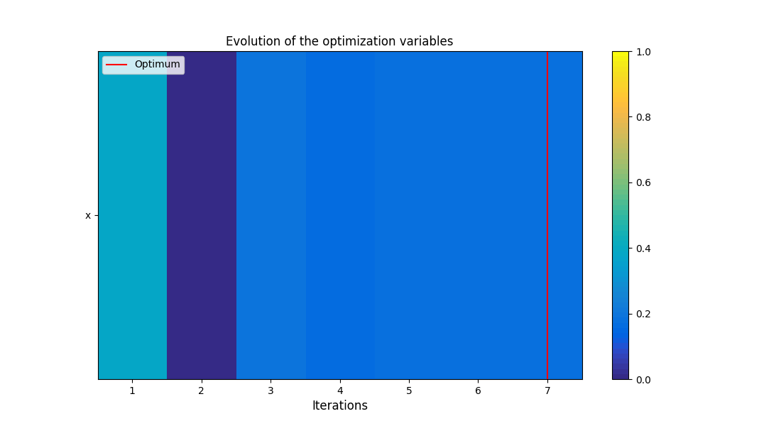
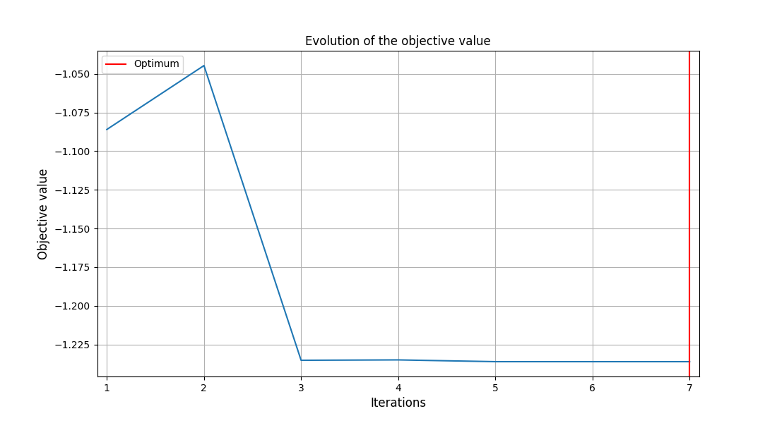
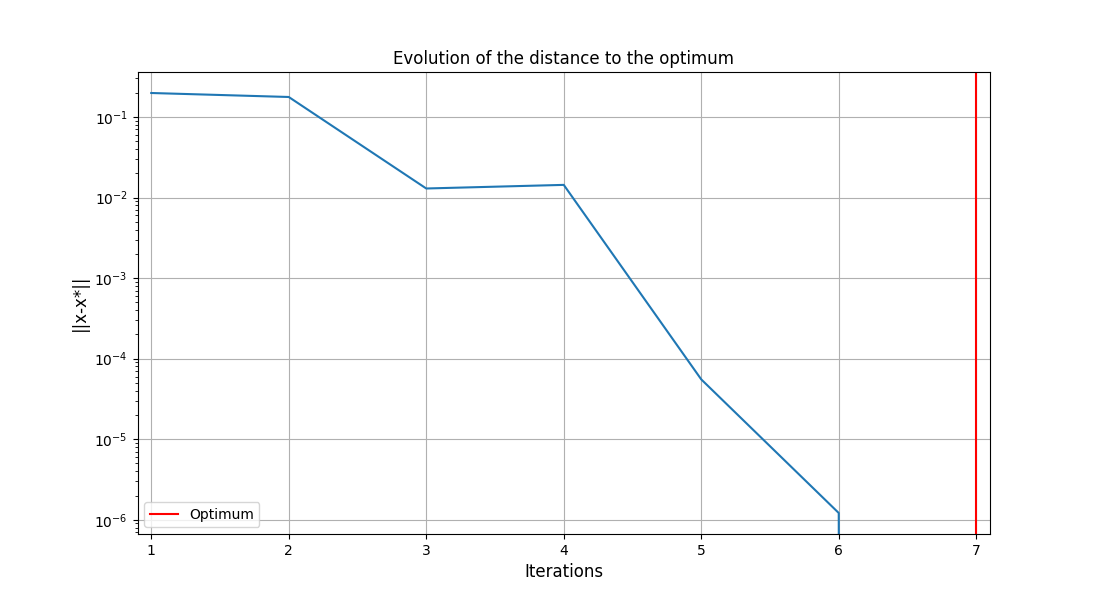
We can also post-process the optimization history by means of the function
execute_post(),
either from the OptimizationProblem:
execute_post(problem, post_name="OptHistoryView", save=False, show=True)

<gemseo.post.opt_history_view.OptHistoryView object at 0x72a4f3128ec0>
or from the HDF file created above:
execute_post("my_optim.hdf5", post_name="OptHistoryView", save=False, show=True)


    INFO - 16:25:02: Importing the optimization problem from the file my_optim.hdf5

<gemseo.post.opt_history_view.OptHistoryView object at 0x72a4d5cbdd30>
Total running time of the script: (0 minutes 0.602 seconds)