Comparing sensitivity indices

from __future__ import annotations

from gemseo.problems.uncertainty.ishigami.ishigami_discipline import IshigamiDiscipline
from gemseo.problems.uncertainty.ishigami.ishigami_space import IshigamiSpace
from gemseo.uncertainty.sensitivity.correlation_analysis import CorrelationAnalysis
from gemseo.uncertainty.sensitivity.morris_analysis import MorrisAnalysis

In this example, we consider the Ishigami function [IH90]

\[f(x_1,x_2,x_3)=\sin(x_1)+7\sin(x_2)^2+0.1x_3^4\sin(x_1)\]

implemented as an Discipline by the IshigamiDiscipline. It is commonly used with the independent random variables \(X_1\), \(X_2\) and \(X_3\) uniformly distributed between \(-\pi\) and \(\pi\) and defined in the IshigamiSpace.

discipline = IshigamiDiscipline()
uncertain_space = IshigamiSpace()

We would like to carry out two sensitivity analyses, e.g. a first one based on correlation coefficients and a second one based on the Morris methodology, and compare the results,

Firstly, we create a CorrelationAnalysis and compute the sensitivity indices:

correlation = CorrelationAnalysis()
correlation.compute_samples([discipline], uncertain_space, 10)
correlation.compute_indices()

    INFO - 16:16:35: *** Start CorrelationAnalysisSamplingPhase execution ***
    INFO - 16:16:35: CorrelationAnalysisSamplingPhase
    INFO - 16:16:35:    Disciplines: IshigamiDiscipline
    INFO - 16:16:35:    MDO formulation: MDF
    INFO - 16:16:35: Running the algorithm OT_MONTE_CARLO:
    INFO - 16:16:35:     10%|█         | 1/10 [00:00<00:00, 418.51 it/sec]
    INFO - 16:16:35:     20%|██        | 2/10 [00:00<00:00, 660.99 it/sec]
    INFO - 16:16:35:     30%|███       | 3/10 [00:00<00:00, 839.42 it/sec]
    INFO - 16:16:35:     40%|████      | 4/10 [00:00<00:00, 985.91 it/sec]
    INFO - 16:16:35:     50%|█████     | 5/10 [00:00<00:00, 1093.69 it/sec]
    INFO - 16:16:35:     60%|██████    | 6/10 [00:00<00:00, 1188.08 it/sec]
    INFO - 16:16:35:     70%|███████   | 7/10 [00:00<00:00, 1261.88 it/sec]
    INFO - 16:16:35:     80%|████████  | 8/10 [00:00<00:00, 1330.68 it/sec]
    INFO - 16:16:35:     90%|█████████ | 9/10 [00:00<00:00, 1378.95 it/sec]
    INFO - 16:16:35:    100%|██████████| 10/10 [00:00<00:00, 1407.06 it/sec]
    INFO - 16:16:35: *** End CorrelationAnalysisSamplingPhase execution ***

CorrelationAnalysis.SensitivityIndices(kendall={'y': [{'x1': array([0.55555556]), 'x2': array([0.02222222]), 'x3': array([-0.11111111])}]}, pcc={'y': [{'x1': array([0.84696461]), 'x2': array([0.68814608]), 'x3': array([-0.29846394])}]}, pearson={'y': [{'x1': array([0.685388]), 'x2': array([0.09681897]), 'x3': array([-0.23027298])}]}, prcc={'y': [{'x1': array([0.90374102]), 'x2': array([0.76539572]), 'x3': array([-0.02232206])}]}, spearman={'y': [{'x1': array([0.74545455]), 'x2': array([0.04242424]), 'x3': array([-0.09090909])}]}, src={'y': [{'x1': array([0.94001308]), 'x2': array([0.55748872]), 'x3': array([-0.16157012])}]}, srrc={'y': [{'x1': array([1.06252802]), 'x2': array([0.60167726]), 'x3': array([-0.00959941])}]}, ssrc={'y': [{'x1': array([0.88362459]), 'x2': array([0.31079367]), 'x3': array([0.0261049])}]})

Then, we create an MorrisAnalysis and compute the sensitivity indices:

morris = MorrisAnalysis()
morris.compute_samples([discipline], uncertain_space, 10)
morris.compute_indices()

    INFO - 16:16:35: *** Start MorrisAnalysisSamplingPhase execution ***
    INFO - 16:16:35: MorrisAnalysisSamplingPhase
    INFO - 16:16:35:    Disciplines: IshigamiDiscipline
    INFO - 16:16:35:    MDO formulation: MDF
    INFO - 16:16:35: Running the algorithm MorrisDOE:
    INFO - 16:16:35:     12%|█▎        | 1/8 [00:00<00:00, 2730.67 it/sec]
    INFO - 16:16:35:     25%|██▌       | 2/8 [00:00<00:00, 2137.22 it/sec]
    INFO - 16:16:35:     38%|███▊      | 3/8 [00:00<00:00, 2036.07 it/sec]
    INFO - 16:16:35:     50%|█████     | 4/8 [00:00<00:00, 1961.33 it/sec]
    INFO - 16:16:35:     62%|██████▎   | 5/8 [00:00<00:00, 1955.02 it/sec]
    INFO - 16:16:35:     75%|███████▌  | 6/8 [00:00<00:00, 1957.67 it/sec]
    INFO - 16:16:35:     88%|████████▊ | 7/8 [00:00<00:00, 1946.05 it/sec]
    INFO - 16:16:35:    100%|██████████| 8/8 [00:00<00:00, 1884.97 it/sec]
    INFO - 16:16:35: *** End MorrisAnalysisSamplingPhase execution ***

MorrisAnalysis.SensitivityIndices(mu={'y': [{'x1': array([0.73532408]), 'x2': array([-0.05115399]), 'x3': array([-1.6024484])}]}, mu_star={'y': [{'x1': array([0.76770333]), 'x2': array([2.09435091]), 'x3': array([1.6024484])}]}, sigma={'y': [{'x1': array([0.76770333]), 'x2': array([2.09435091]), 'x3': array([1.58984353])}]}, relative_sigma={'y': [{'x1': array([1.]), 'x2': array([1.]), 'x3': array([0.99213399])}]}, min={'y': [{'x1': array([0.03237925]), 'x2': array([2.04319692]), 'x3': array([0.01260487])}]}, max={'y': [{'x1': array([1.50302741]), 'x2': array([2.14550491]), 'x3': array([3.19229192])}]})

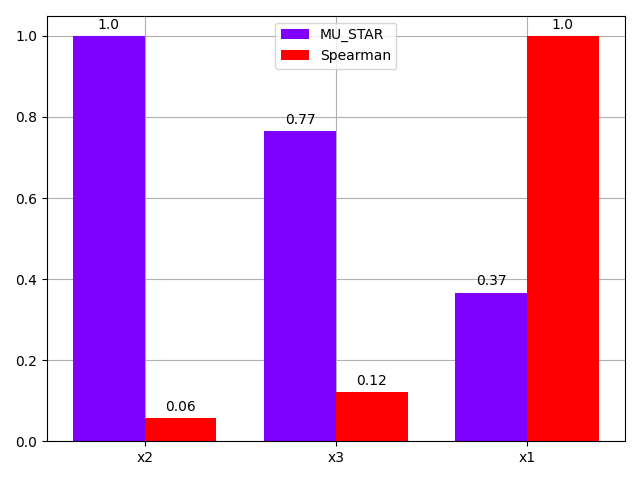
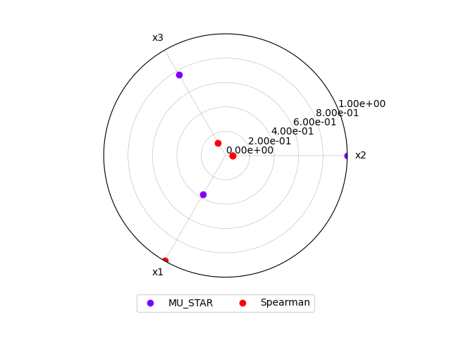
Lastly, we compare these analyses with the graphical method BaseSensitivityAnalysis.plot_comparison(), either using a bar chart:

morris.plot_comparison(correlation, "y", use_bar_plot=True, save=False, show=True)

<gemseo.post.dataset.bars.BarPlot object at 0x7b1d380539b0>

or a radar plot:

morris.plot_comparison(correlation, "y", use_bar_plot=False, save=False, show=True)

<gemseo.post.dataset.radar_chart.RadarChart object at 0x7b1d38fca0c0>

Tip

The comparison method can use plotly to generate an interactive web-based figure. Just set the execution option file_format to "html".