analysis module¶

Abstract class for the computation and analysis of sensitivity indices.

The purpose of a sensitivity analysis is to qualify or quantify how the model’s uncertain inputs impact its outputs.

This analysis relies on BaseSensitivityAnalysis computed from a MDODiscipline representing the model, a ParameterSpace describing the uncertain parameters and options associated with a particular concrete class inheriting from BaseSensitivityAnalysis which is an abstract one.

class gemseo.uncertainty.sensitivity.analysis.BaseSensitivityAnalysis(disciplines, parameter_space, n_samples=None, output_names=(), algo='', algo_options=mappingproxy({}), formulation='MDF', **formulation_options)[source]¶

Bases: object

Sensitivity analysis.

The BaseSensitivityAnalysis class provides both the values of BaseSensitivityAnalysis.indices and their graphical representations, from either the plot() method, the plot_radar() method or the plot_bar() method.

It is also possible to use sort_parameters() to get the parameters sorted according to main_method. The main_indices are indices computed with the latter.

Lastly, the plot_comparison() method allows to compare the current BaseSensitivityAnalysis with another one.

Parameters:

disciplines (Collection[MDODiscipline]) – The discipline or disciplines to use for the analysis.
parameter_space (ParameterSpace) – A parameter space.
n_samples (int | None) – A number of samples. If None, the number of samples is computed by the algorithm.
output_names (Iterable[str]) –
The disciplines’ outputs to be considered for the analysis. If empty, use all the outputs.

By default it is set to ().
algo (str) –
The name of the DOE algorithm. If empty, use the BaseSensitivityAnalysis.DEFAULT_DRIVER.

By default it is set to “”.
algo_options (Mapping[str, DOELibraryOptionType]) –
The options of the DOE algorithm.

By default it is set to {}.
formulation (str) –
The name of the MDOFormulation to sample the disciplines.

By default it is set to “MDF”.
**formulation_options (Any) – The options of the MDOFormulation.

abstract compute_indices(outputs=())[source]¶

Compute the sensitivity indices.

Parameters:

outputs (str | Sequence[str]) –

The name(s) of the output(s) for which to compute the sensitivity indices. If empty, use the names of the outputs set at instantiation.

By default it is set to ().

Returns:

The sensitivity indices.

With the following structure:

{
    "method_name": {
        "output_name": [
            {
                "input_name": data_array,
            }
        ]
    }
}

Return type:

dict[str, FirstOrderIndicesType | SecondOrderIndicesType]

static from_pickle(file_path)[source]¶

Load a sensitivity analysis from the disk.

Parameters:: file_path (str | Path) – The path to the file.
Returns:: The sensitivity analysis.
Return type:: BaseSensitivityAnalysis

plot(output, inputs=(), title='', save=True, show=False, file_path='', file_format='')[source]¶

Plot the sensitivity indices.

Parameters:

output (VariableType) – The output for which to display sensitivity indices, either a name or a tuple of the form (name, component). If name, its first component is considered.
inputs (Iterable[str]) –
The uncertain input variables for which to display the sensitivity indices. If empty, display all the uncertain input variables.

By default it is set to ().
title (str) –
The title of the plot, if any.

By default it is set to “”.
save (bool) –
If True, save the figure.

By default it is set to True.
show (bool) –
If True, show the figure.

By default it is set to False.
file_path (str | Path) –
A file path. Either a complete file path, a directory name or a file name. If empty, use a default file name and a default directory. The file extension is inferred from filepath extension, if any.

By default it is set to “”.
file_format (str) –
A file format, e.g. ‘png’, ‘pdf’, ‘svg’, … Used when file_path does not have any extension. If empty, use a default file extension.

By default it is set to “”.

Returns:

The plot figure.

Return type:

DatasetPlot | Figure

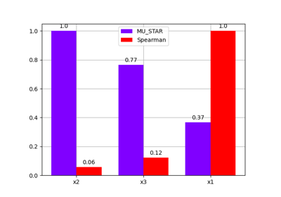
plot_bar(outputs=(), inputs=(), standardize=False, title='', save=True, show=False, file_path='', directory_path='', file_name='', file_format='', sort=True, sorting_output='', **options)[source]¶

Plot the sensitivity indices on a bar chart.

This method may consider one or more outputs, as well as all inputs (default behavior) or a subset.

Parameters:

outputs (OutputsType) –
The outputs for which to display sensitivity indices, either a name, a list of names, a (name, component) tuple, a list of such tuples or a list mixing such tuples and names. When a name is specified, all its components are considered. If empty, use the default outputs.

By default it is set to ().
inputs (Iterable[str]) –
The uncertain input variables for which to display the sensitivity indices. If empty, display all the uncertain input variables.

By default it is set to ().
standardize (bool) –
Whether to scale the indices to \([0,1]\).

By default it is set to False.
title (str) –
The title of the plot, if any.

By default it is set to “”.
save (bool) –
If True, save the figure.

By default it is set to True.
show (bool) –
If True, show the figure.

By default it is set to False.
file_path (str | Path) –
The path of the file to save the figures. If the extension is missing, use file_extension. If empty, create a file path from directory_path, file_name and file_extension.

By default it is set to “”.
directory_path (str | Path) –
The path of the directory to save the figures. If empty, use the current working directory.

By default it is set to “”.
file_name (str) –
The name of the file to save the figures. If empty, use a default one generated by the post-processing.

By default it is set to “”.
file_format (str) –
A file extension, e.g. ‘png’, ‘pdf’, ‘svg’, … If None, use a default file extension.

By default it is set to “”.
**options (int) – The options to instantiate the BarPlot. If empty, use a default file extension.
sort (bool) –
Whether to sort the uncertain variables by decreasing order of the sensitivity indices associated with the sorting output variable.

By default it is set to True.
sorting_output (VariableType) –
The sorting output variable If empty, use the first one.

By default it is set to “”.
**options – The options to instantiate the BarPlot.

Returns:

A bar chart representing the sensitivity indices.

Return type:

BarPlot

plot_comparison(indices, output, inputs=(), title='', use_bar_plot=True, save=True, show=False, file_path='', directory_path='', file_name='', file_format='', **options)[source]¶

Plot a comparison between the current sensitivity indices and other ones.

This method allows to use either a bar chart (default option) or a radar one.

Parameters:

indices (list[BaseSensitivityAnalysis]) – The sensitivity indices.
output (VariableType) – The output for which to display sensitivity indices, either a name or a tuple of the form (name, component). If name, its first component is considered.
inputs (Iterable[str]) –
The uncertain input variables for which to display the sensitivity indices. If empty, display all the uncertain input variables.

By default it is set to ().
title (str) –
The title of the plot, if any.

By default it is set to “”.
use_bar_plot (bool) –
The type of graph. If True, use a bar plot. Otherwise, use a radar chart.

By default it is set to True.
save (bool) –
If True, save the figure.

By default it is set to True.
show (bool) –
If True, show the figure.

By default it is set to False.
file_path (str | Path) –
The path of the file to save the figures. If empty, create a file path from directory_path, file_name and file_format.

By default it is set to “”.
directory_path (str | Path) –
The path of the directory to save the figures. If empty, use the current working directory.

By default it is set to “”.
file_name (str) –
The name of the file to save the figures. If empty, use a default one generated by the post-processing.

By default it is set to “”.
file_format (str) –
A file format, e.g. ‘png’, ‘pdf’, ‘svg’, … If empty, use a default file extension.

By default it is set to “”.
**options (bool) – The options passed to the underlying DatasetPlot.

Returns:

A graph comparing sensitivity indices.

Return type:

BarPlot | RadarChart

plot_field(output, mesh=None, inputs=(), standardize=False, title='', save=True, show=False, file_path='', directory_path='', file_name='', file_format='', properties=mappingproxy({}))[source]¶

Plot the sensitivity indices related to a 1D or 2D functional output.

The output is considered as a 1D or 2D functional variable, according to the shape of the mesh on which it is represented.

Parameters:

output (VariableType) – The output for which to display sensitivity indices, either a name or a tuple of the form (name, component) where (name, component) is used to sort the inputs. If it is a name, its first component is considered.
mesh (ndarray | None) – The mesh on which the p-length output is represented. Either a p-length array for a 1D functional output or a (p, 2) array for a 2D one. If None, assume a 1D functional output.
inputs (Iterable[str]) –
The uncertain input variables for which to display the sensitivity indices. If empty, display all the uncertain input variables.

By default it is set to ().
standardize (bool) –
Whether to scale the indices to \([0,1]\).

By default it is set to False.
title (str) –
The title of the plot, if any.

By default it is set to “”.
save (bool) –
If True, save the figure.

By default it is set to True.
show (bool) –
If True, show the figure.

By default it is set to False.
file_path (str | Path) –
The path of the file to save the figures. If empty, create a file path from directory_path, file_name and file_extension.

By default it is set to “”.
directory_path (str | Path) –
The path of the directory to save the figures. If empty, use the current working directory.

By default it is set to “”.
file_name (str) –
The name of the file to save the figures. If empty, use a default one generated by the post-processing.

By default it is set to “”.
file_format (str) –
A file extension, e.g. ‘png’, ‘pdf’, ‘svg’, … If empty, use a default file extension.

By default it is set to “”.
properties (Mapping[str, DatasetPlotPropertyType]) –
The general properties of a DatasetPlot.

By default it is set to {}.

Returns:

A bar plot representing the sensitivity indices.

Raises:

NotImplementedError – If the dimension of the mesh is greater than 2.

Return type:

Curves | Surfaces

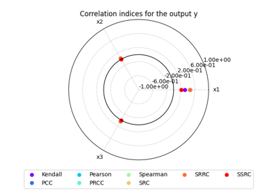
plot_radar(outputs=(), inputs=(), standardize=False, title='', save=True, show=False, file_path='', directory_path='', file_name='', file_format='', min_radius=None, max_radius=None, sort=True, sorting_output='', **options)[source]¶

Plot the sensitivity indices on a radar chart.

This method may consider one or more outputs, as well as all inputs (default behavior) or a subset.

For visualization purposes, it is also possible to change the minimum and maximum radius values.

Parameters:

outputs (OutputsType) –
The outputs for which to display sensitivity indices, either a name, a list of names, a (name, component) tuple, a list of such tuples or a list mixing such tuples and names. When a name is specified, all its components are considered. If empty, use the default outputs.

By default it is set to ().
inputs (Iterable[str]) –
The uncertain input variables for which to display the sensitivity indices. If empty, display all the uncertain input variables.

By default it is set to ().
standardize (bool) –
Whether to scale the indices to \([0,1]\).

By default it is set to False.
title (str) –
The title of the plot, if any.

By default it is set to “”.
save (bool) –
If True, save the figure.

By default it is set to True.
show (bool) –
If True, show the figure.

By default it is set to False.
file_path (str | Path) –
The path of the file to save the figures. If the extension is missing, use file_extension. If empty, create a file path from directory_path, file_name and file_extension.

By default it is set to “”.
directory_path (str | Path) –
The path of the directory to save the figures. If empty, use the current working directory.

By default it is set to “”.
file_name (str) –
The name of the file to save the figures. If empty, use a default one generated by the post-processing.

By default it is set to “”.
file_format (str) –
A file extension, e.g. ‘png’, ‘pdf’, ‘svg’, … If empty, use a default file extension.

By default it is set to “”.
min_radius (float | None) – The minimal radial value. If None, from data.
max_radius (float | None) – The maximal radial value. If None, from data.
sort (bool) –
Whether to sort the uncertain variables by decreasing order of the sensitivity indices associated with the sorting output variable.

By default it is set to True.
sorting_output (VariableType) –
The sorting output variable If empty, use the first one.

By default it is set to “”.
**options (bool | int) – The options to instantiate the RadarChart.

Returns:

A radar chart representing the sensitivity indices.

Return type:

RadarChart

sort_parameters(output)[source]¶

Return the parameters sorted in descending order.

Parameters:: output (VariableType) – Either a tuple as (output_name, output_component) or an output name; in the second case, use the first output component.
Returns:: The input parameters sorted by decreasing order of sensitivity; in case of a multivariate input, aggregate the sensitivity indices associated to the different input components by adding them up typically.
Return type:: list[str]

static standardize_indices(indices)[source]¶

Standardize the sensitivity indices for each output component.

Each index is replaced by its absolute value divided by the largest index. Thus, the standardized indices belong to the interval \([0,1]\).

Parameters:: indices (dict[str, list[dict[str, ndarray]]]) – The indices to be standardized.
Returns:: The standardized indices.
Return type:: dict[str, list[dict[str, ndarray]]]

to_dataset()[source]¶

Convert BaseSensitivityAnalysis.indices into a Dataset.

Returns:: The sensitivity indices.
Return type:: Dataset

to_pickle(file_path)[source]¶

Save the current sensitivity analysis on the disk.

Parameters:: file_path (str | Path) – The path to the file.
Return type:: None

DEFAULT_DRIVER = None¶

Method: ClassVar[type[StrEnum]]¶

The names of the sensitivity methods considering simple effects.

A simple effect is the effect of an isolated input variable on an output variable while an interaction effect is the effect of the interaction between several input variables on an output variable.

dataset: IODataset¶: The dataset containing the discipline evaluations.

default_output: Iterable[str]¶: The default outputs of interest.

property indices: dict[str, dict[str, list[dict[str, ndarray]]]]¶

The sensitivity indices.

With the following structure:

{
    "method_name": {
        "output_name": [
            {
                "input_name": data_array,
            }
        ]
    }
}

property input_names: list[str]¶: The names of the inputs.

property main_indices: dict[str, list[dict[str, ndarray]]]¶

The main sensitivity indices.

With the following structure:

{
    "output_name": [
        {
            "input_name": data_array,
        }
    ]
}

property main_method: Method¶

The name of the main method.

One of the enum Sensitivity.Method.

Examples using BaseSensitivityAnalysis¶

Comparing sensitivity indices

Correlation analysis

Morris analysis

Sobol’ analysis

Sobol' analysis