gemseo / uncertainty / sensitivity / sobol

analysis module¶

Class for the estimation of Sobol’ indices.

Let us consider the model \(Y=f(X_1,\ldots,X_d)\) where:

\(X_1,\ldots,X_d\) are independent random variables,
\(E\left[f(X_1,\ldots,X_d)^2\right]<\infty\).

Then, the following decomposition is unique:

\[Y=f_0 + \sum_{i=1}^df_i(X_i) + \sum_{i,j=1\atop i\neq j}^d f_{i,j}(X_i,X_j) + \sum_{i,j,k=1\atop i\neq j\neq k}^d f_{i,j,k}(X_i,X_j,X_k) + \ldots + f_{1,\ldots,d}(X_1,\ldots,X_d)\]

where:

\(f_0=E[Y]\),
\(f_i(X_i)=E[Y|X_i]-f_0\),
\(f_{i,j}(X_i,X_j)=E[Y|X_i,X_j]-f_i(X_i)-f_j(X_j)-f_0\)
and so on.

Then, the shift to variance leads to:

\[V[Y]=\sum_{i=1}^dV\left[f_i(X_i)\right] + \sum_{i,j=1\atop j\neq i}^d V\left[f_{i,j}(X_i,X_j)\right] + \ldots + V\left[f_{1,\ldots,d}(X_1,\ldots,X_d)\right]\]

and the Sobol’ indices are obtained by dividing by the variance and sum up to 1:

\[1=\sum_{i=1}^dS_i + \sum_{i,j=1\atop j\neq i}^d S_{i,j} + \sum_{i,j,k=1\atop i\neq j\neq k}^d S_{i,j,k} + \ldots + S_{1,\ldots,d}\]

A Sobol’ index represents the share of output variance explained by a parameter or a group of parameters. For the parameter \(X_i\),

\(S_i\) is the first-order Sobol’ index measuring the individual effect of \(X_i\),
\(S_{i,j}\) is the second-order Sobol’ index measuring the joint effect between \(X_i\) and \(X_j\),
\(S_{i,j,k}\) is the third-order Sobol’ index measuring the joint effect between \(X_i\), \(X_j\) and \(X_k\),
and so on.

In practice, we only consider the first-order Sobol’ index:

\[S_i=\frac{V[E[Y|X_i]]}{V[Y]}\]

and the total-order Sobol’ index:

\[S_i^T=\sum_{u\subset\{1,\ldots,d\}\atop u \ni i}S_u\]

The latter represents the sum of the individual effect of \(X_i\) and the joint effects between \(X_i\) and any parameter or group of parameters.

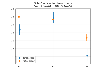
This methodology relies on the SobolAnalysis class. Precisely, SobolAnalysis.indices contains both SobolAnalysis.first_order_indices and SobolAnalysis.total_order_indices while SobolAnalysis.main_indices represents total-order Sobol’ indices. Lastly, the SobolAnalysis.plot() method represents the estimations of both first-order and total-order Sobol’ indices along with their confidence intervals whose default level is 95%.

The user can select the algorithm to estimate the Sobol’ indices. The computation relies on OpenTURNS capabilities.

class gemseo.uncertainty.sensitivity.sobol.analysis.SobolAnalysis(disciplines, parameter_space, n_samples, output_names=(), algo='', algo_options=mappingproxy({}), formulation='MDF', compute_second_order=True, use_asymptotic_distributions=True, **formulation_options)[source]

Bases: SensitivityAnalysis

Sensitivity analysis based on the Sobol’ indices.

Examples

>>> from numpy import pi
>>> from gemseo import create_discipline, create_parameter_space
>>> from gemseo.uncertainty.sensitivity.sobol.analysis import SobolAnalysis
>>>
>>> expressions = {"y": "sin(x1)+7*sin(x2)**2+0.1*x3**4*sin(x1)"}
>>> discipline = create_discipline(
...     "AnalyticDiscipline", expressions=expressions
... )
>>>
>>> parameter_space = create_parameter_space()
>>> parameter_space.add_random_variable(
...     "x1", "OTUniformDistribution", minimum=-pi, maximum=pi
... )
>>> parameter_space.add_random_variable(
...     "x2", "OTUniformDistribution", minimum=-pi, maximum=pi
... )
>>> parameter_space.add_random_variable(
...     "x3", "OTUniformDistribution", minimum=-pi, maximum=pi
... )
>>>
>>> analysis = SobolAnalysis([discipline], parameter_space, n_samples=10000)
>>> indices = analysis.compute_indices()

Parameters:

disciplines (Collection[MDODiscipline]) – The discipline or disciplines to use for the analysis.
parameter_space (ParameterSpace) – A parameter space.
n_samples (int) – A number of samples. If None, the number of samples is computed by the algorithm.
output_names (Iterable[str]) –
The disciplines’ outputs to be considered for the analysis. If empty, use all the outputs.

By default it is set to ().
algo (str) –
The name of the DOE algorithm. If empty, use the SensitivityAnalysis.DEFAULT_DRIVER.

By default it is set to “”.
algo_options (Mapping[str, DOELibraryOptionType]) –
The options of the DOE algorithm.

By default it is set to {}.
formulation (str) –
The name of the MDOFormulation to sample the disciplines.

By default it is set to “MDF”.
compute_second_order (bool) –
Whether to compute the second-order indices.

By default it is set to True.
use_asymptotic_distributions (bool) –
Whether to estimate the confidence intervals of the first- and total-order Sobol’ indices with the asymptotic distributions; otherwise, use bootstrap.

By default it is set to True.
**formulation_options (Any) – The options of the MDOFormulation.

Notes

The estimators of Sobol’ indices rely on the same DOE algorithm. This algorithm starts with two independent input datasets composed of \(N\) independent samples and this number \(N\) is the usual sampling size for Sobol’ analysis. When compute_second_order=False or when the input dimension \(d\) is equal to 2, \(N=\frac{n_\text{samples}}{2+d}\). Otherwise, \(N=\frac{n_\text{samples}}{2+2d}\). The larger \(N\), the more accurate the estimators of Sobol’ indices are. Therefore, for a small budget n_samples, the user can choose to set compute_second_order to False to ensure a better estimation of the first- and second-order indices.

class Algorithm(value)[source]

Bases: PascalCaseStrEnum

The algorithms to estimate the Sobol’ indices.

JANSEN = 'Jansen'

MARTINEZ = 'Martinez'

MAUNTZ_KUCHERENKO = 'MauntzKucherenko'

SALTELLI = 'Saltelli'

class Method(value)[source]

Bases: StrEnum

The names of the sensitivity methods.

FIRST = 'first': The first-order Sobol’ index.

TOTAL = 'total': The total-order Sobol’ index.

compute_indices(outputs=(), algo=Algorithm.SALTELLI, confidence_level=0.95)[source]

Compute the sensitivity indices.

Parameters:

outputs (str | Sequence[str]) –
The name(s) of the output(s) for which to compute the sensitivity indices. If empty, use the names of the outputs set at instantiation.

By default it is set to ().
algo (Algorithm) –
The name of the algorithm to estimate the Sobol’ indices.

By default it is set to “Saltelli”.
confidence_level (float) –
The level of the confidence intervals.

By default it is set to 0.95.

Returns:

The sensitivity indices.

With the following structure:

{
    "method_name": {
        "output_name": [
            {
                "input_name": data_array,
            }
        ]
    }
}

Return type:

dict[str, FirstOrderIndicesType]

get_intervals(first_order=True)[source]

Get the confidence intervals for the Sobol’ indices.

Warning

You must first call compute_indices().

Parameters:

first_order (bool) –

If True, compute the intervals for the first-order indices. Otherwise, for the total-order indices.

By default it is set to True.

Returns:

The confidence intervals for the Sobol’ indices.

With the following structure:

{
    "output_name": [
        {
            "input_name": data_array,
        }
    ]
}

Return type:

dict[str, list[dict[str, ndarray]]]

plot(output, inputs=(), title='', save=True, show=False, file_path='', directory_path='', file_name='', file_format='', sort=True, sort_by_total=True)[source]

Plot the first- and total-order Sobol’ indices.

For the \(i\)-th uncertain input variable, plot its first-order Sobol’ index \(S_i^{1}\) and its total-order Sobol’ index \(S_i^{T}\) with dots and their confidence intervals with vertical lines.

The subtitle displays the standard deviation (StD) and the variance (Var) of the output of interest.

Parameters:

output (VariableType) – The output for which to display sensitivity indices, either a name or a tuple of the form (name, component). If name, its first component is considered.
inputs (Iterable[str]) –
The uncertain input variables for which to display the sensitivity indices. If empty, display all the uncertain input variables.

By default it is set to ().
title (str) –
The title of the plot. If empty, use a default one.

By default it is set to “”.
save (bool) –
If True, save the figure.

By default it is set to True.
show (bool) –
If True, show the figure.

By default it is set to False.
file_path (str | Path) –
A file path. Either a complete file path, a directory name or a file name. If empty, use a default file name and a default directory. The file extension is inferred from filepath extension, if any.

By default it is set to “”.
directory_path (str | Path) –
The path to the directory where to save the plots.

By default it is set to “”.
file_name (str) –
The name of the file.

By default it is set to “”.
file_format (str) –
A file format, e.g. ‘png’, ‘pdf’, ‘svg’, … Used when file_path does not have any extension. If empty, use a default file extension.

By default it is set to “”.
sort (bool) –
Whether to sort the uncertain variables by decreasing order.

By default it is set to True.
sort_by_total (bool) –
Whether to sort according to the total-order Sobol’ indices when sort is True. Otherwise, use the first-order Sobol’ indices.

By default it is set to True.

Returns:

The plot figure.

Return type:

Figure

unscale_indices(indices, use_variance=True)[source]

Unscale the Sobol’ indices.

Parameters:

indices (FirstOrderIndicesType | SecondOrderIndicesType) – The Sobol’ indices.
use_variance (bool) –
Whether to express an unscaled Sobol’ index as a share of output variance; otherwise, express it as the square root of this part and therefore with the same unit as the output.

By default it is set to True.

Returns:

The unscaled Sobol’ indices.

Return type:

FirstOrderIndicesType | SecondOrderIndicesType

DEFAULT_DRIVER: ClassVar[str] = 'OT_SOBOL_INDICES'

dataset: IODataset: The dataset containing the discipline evaluations.

default_output: Iterable[str]: The default outputs of interest.

property first_order_indices: dict[str, list[dict[str, ndarray]]]

The first-order Sobol’ indices.

With the following structure:

{
    "output_name": [
        {
            "input_name": data_array,
        }
    ]
}

output_standard_deviations: dict[str, NDArray[float]]: The standard deviations of the output variables.

output_variances: dict[str, NDArray[float]]: The variances of the output variables.

property second_order_indices: dict[str, list[dict[str, dict[str, ndarray]]]]

The second-order Sobol’ indices.

With the following structure:

{
    "output_name": [
        {
            {"input_name": {"other_input_name": data_array},
        }
    ]
}

property total_order_indices: dict[str, list[dict[str, ndarray]]]

The total-order Sobol’ indices.

With the following structure:

{
    "output_name": [
        {
            "input_name": data_array,
        }
    ]
}

Examples using SobolAnalysis¶

Sobol’ analysis

Sobol' analysis