empirical module¶

Class for the empirical estimation of statistics from a dataset.

Overview¶

The EmpiricalStatistics class inherits from the abstract Statistics class and aims to estimate statistics from a Dataset, based on empirical estimators.

Construction¶

A EmpiricalStatistics is built from a Dataset and optionally variables names. In this case, statistics are only computed for these variables. Otherwise, statistics are computed for all the variable available in the dataset. Lastly, the user can give a name to its EmpiricalStatistics object. By default, this name is the concatenation of ‘EmpiricalStatistics’ and the name of the Dataset.

class gemseo.uncertainty.statistics.empirical.EmpiricalStatistics(dataset, variable_names=(), name='')[source]

Bases: Statistics

A toolbox to compute statistics empirically.

Unless otherwise stated, the statistics are computed variable-wise and component-wise, i.e. variable-by-variable and component-by-component. So, for the sake of readability, the methods named as compute_statistic() return dict[str, ndarray] objects whose values are the names of the variables and the values are the statistic estimated for the different component.

Examples

>>> from gemseo import (
...     create_discipline,
...     create_parameter_space,
...     create_scenario,
... )
>>> from gemseo.uncertainty.statistics.empirical import EmpiricalStatistics
>>>
>>> expressions = {"y1": "x1+2*x2", "y2": "x1-3*x2"}
>>> discipline = create_discipline(
...     "AnalyticDiscipline", expressions=expressions
... )
>>>
>>> parameter_space = create_parameter_space()
>>> parameter_space.add_random_variable(
...     "x1", "OTUniformDistribution", minimum=-1, maximum=1
... )
>>> parameter_space.add_random_variable(
...     "x2", "OTUniformDistribution", minimum=-1, maximum=1
... )
>>>
>>> scenario = create_scenario(
...     [discipline],
...     "DisciplinaryOpt",
...     "y1",
...     parameter_space,
...     scenario_type="DOE",
... )
>>> scenario.execute({"algo": "OT_MONTE_CARLO", "n_samples": 100})
>>>
>>> dataset = scenario.to_dataset(opt_naming=False)
>>>
>>> statistics = EmpiricalStatistics(dataset)
>>> mean = statistics.compute_mean()

Parameters:

dataset (Dataset) – A dataset.
variable_names (Iterable[str]) –
The names of the variables for which to compute statistics. If empty, consider all the variables of the dataset.

By default it is set to ().
name (str) –
A name for the toolbox computing statistics. If empty, concatenate the names of the dataset and the name of the class.

By default it is set to “”.

compute_joint_probability(thresh, greater=True)[source]

Compute the joint probability related to a threshold.

Either \(\mathbb{P}[X \geq x]\) or \(\mathbb{P}[X \leq x]\).

Parameters:

thresh (Mapping[str, float | ndarray]) – A threshold \(x\) per variable.
greater (bool) –
The type of probability. If True, compute the probability of exceeding the threshold. Otherwise, compute the opposite.

By default it is set to True.

Returns:

The joint probability of the different variables (by definition of the joint probability, this statistics is not computed component-wise).

Return type:

dict[str, float]

compute_maximum()[source]

Compute the maximum \(\text{Max}[X]\).

Returns:: The component-wise maximum of the different variables.
Return type:: dict[str, ndarray]

compute_mean()[source]

Compute the mean \(\mathbb{E}[X]\).

Returns:: The component-wise mean of the different variables.
Return type:: dict[str, ndarray]

compute_minimum()[source]

Compute the \(\text{Min}[X]\).

Returns:: The component-wise minimum of the different variables.
Return type:: dict[str, ndarray]

compute_moment(order)[source]

Compute the n-th moment \(M[X; n]\).

Parameters:: order (int) – The order \(n\) of the moment.
Returns:: The component-wise moment of the different variables.
Return type:: dict[str, ndarray]

compute_probability(thresh, greater=True)[source]

Compute the probability related to a threshold.

Either \(\mathbb{P}[X \geq x]\) or \(\mathbb{P}[X \leq x]\).

Parameters:

thresh (Mapping[str, float | ndarray]) – A threshold \(x\) per variable.
greater (bool) –
The type of probability. If True, compute the probability of exceeding the threshold. Otherwise, compute the opposite.

By default it is set to True.

Returns:

The component-wise probability of the different variables.

Return type:

dict[str, ndarray]

compute_quantile(prob)[source]

Compute the quantile \(\mathbb{Q}[X; \alpha]\) related to a probability.

Parameters:: prob (float) – A probability \(\alpha\) between 0 and 1.
Returns:: The component-wise quantile of the different variables.
Return type:: dict[str, ndarray]

compute_range()[source]

Compute the range \(R[X]\).

Returns:: The component-wise range of the different variables.
Return type:: dict[str, ndarray]

compute_standard_deviation()[source]

Compute the standard deviation \(\mathbb{S}[X]\).

Returns:: The component-wise standard deviation of the different variables.
Return type:: dict[str, ndarray]

compute_variance()[source]

Compute the variance \(\mathbb{V}[X]\).

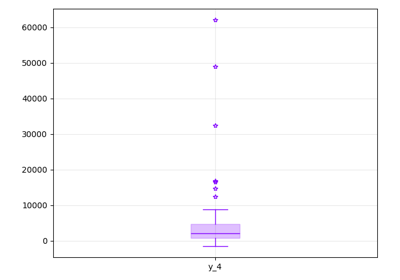
Returns:: The component-wise variance of the different variables.
Return type:: dict[str, ndarray]

plot_boxplot(save=False, show=True, directory_path='', file_format='png', **options)[source]

Visualize the data with a boxplot.

Parameters:

save (bool) –
Whether to save the figures.

By default it is set to False.
show (bool) –
Whether to show the figures.

By default it is set to True.
directory_path (str | Path) –
The path to save the figures.

By default it is set to “”.
file_format (str) –
The file extension.

By default it is set to “png”.
**options (Any) – The options of the Boxplot graphs.

Returns:

The boxplot of each variable.

Return type:

dict[str, Boxplot]

plot_cdf(save=False, show=True, directory_path='', file_format='png', **options)[source]

Visualize the empirical cumulative probability function.

Parameters:

save (bool) –
Whether to save the figures.

By default it is set to False.
show (bool) –
Whether to show the figures.

By default it is set to True.
directory_path (str | Path) –
The path to save the figures.

By default it is set to “”.
file_format (str) –
The file extension.

By default it is set to “png”.
**options (Any) – The options of the Lines graphs.

Returns:

The graph of the cumulative probability function for each variable.

Return type:

dict[str, Lines]

plot_pdf(save=False, show=True, directory_path='', file_format='png', **options)[source]

Visualize the empirical probability density function.

Parameters:

save (bool) –
Whether to save the figures.

By default it is set to False.
show (bool) –
Whether to show the figures.

By default it is set to True.
directory_path (str | Path) –
The path to save the figures.

By default it is set to “”.
file_format (str) –
The file extension.

By default it is set to “png”.
**options (Any) – The options of the Lines graphs.

Returns:

The graph of the probability density function for each variable.

Return type:

dict[str, Lines]

dataset: Dataset: The dataset.

n_samples: int: The number of samples.

n_variables: int: The number of variables.

name: str: The name of the object.

Examples using EmpiricalStatistics¶

Empirical estimation of statistics