Correlations

A correlation coefficient indicates whether there is a linear relationship between 2 quantities \(x\) and \(y\), in which case it equals 1 or -1. It is the normalized covariance between the two quantities:

\[R_{xy}=\frac {\sum \limits _{i=1}^n(x_i-{\bar{x}})(y_i-{\bar{y}})}{ns_{x}s_{y}}= \frac {\sum \limits _{i=1}^n(x_i-{\bar{x}})(y_i-{\bar{y}})}{\sqrt {\sum \limits _{i=1}^n(x_i-{\bar{x}})^{2}\sum \limits _{i=1}^n(y_i-{\bar{y}})^{2}}}\]

To compute the correlations between all inputs and all outputs as well as between two outputs, use the API method execute_post() with the keyword “Correlations” and additional arguments concerning the type of display (file, screen, both):

scenario.post_process(“Correlations”, coeff_limit=0.85, save=True,
show=False, n_plots_x=4, n_plots_y=4)

where:

• coeff_limit is the absolute threshold for correlation plots. It filters the minimum correlation coefficient to be displayed,

• n_plot_x and n_plot_y are the numbers of plots along the columns and the rows, respectively.

Correlation coefficients on the Sobieski use case for the MDF formulation

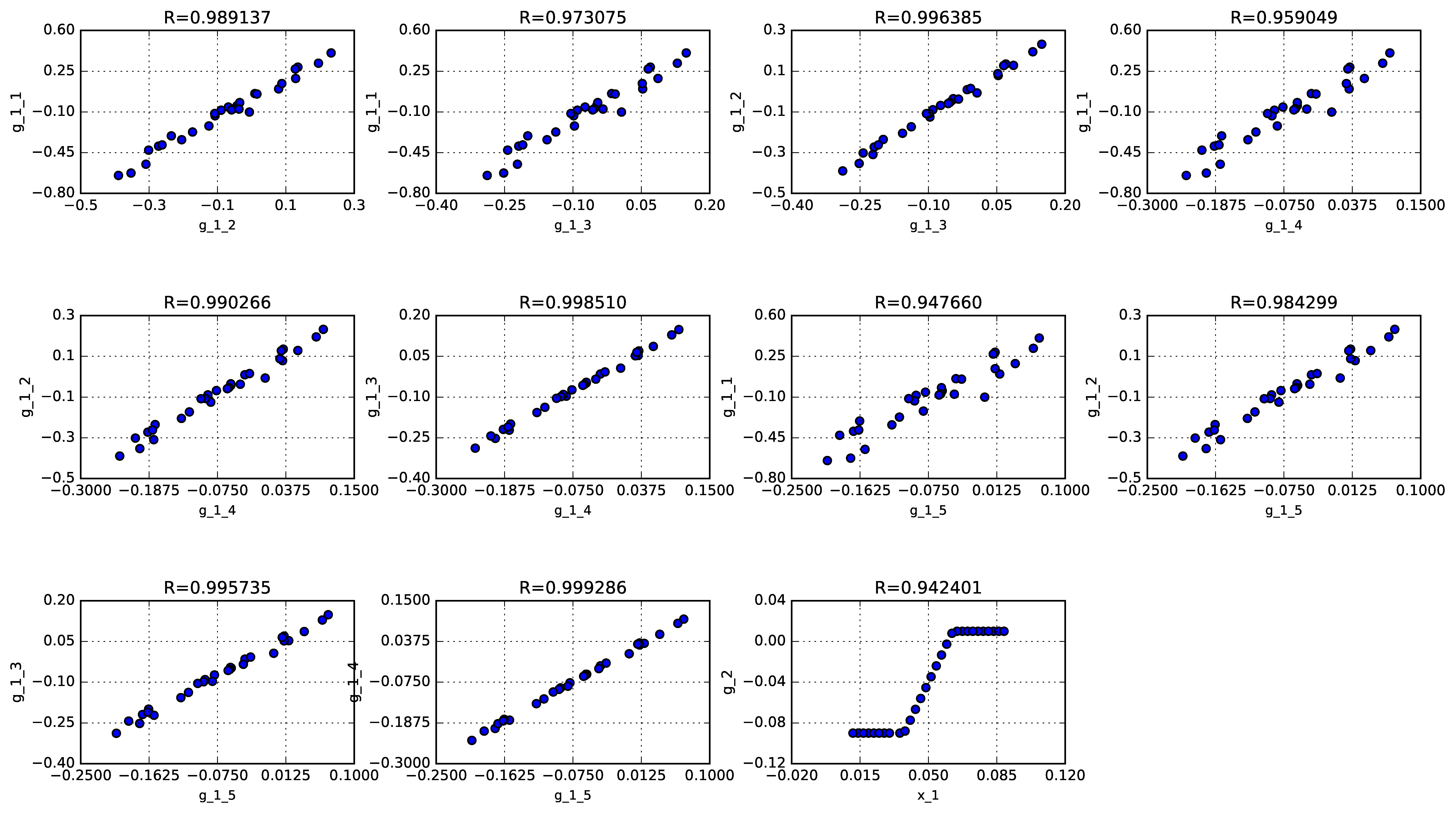
As mentioned earlier, correlation plots highlight the strong correlations between stress constraints in wing sections : the correlation coefficients belong to \([0.94766, 0.999286]\).

The aerodynamics constraint g_2 is a polynomial function of \(x_1\): \(g\_2=1+0.2\overline{x_1}\) with \(\overline{x_1}\) the normalized value of \(x_1\).