Gradient sensitivity

Preliminaries: instantiation and execution of the MDO scenario

Let’s start with the following code lines which instantiate and execute the MDOScenario :

from gemseo.api import create_discipline, create_scenario

formulation = 'MDF'

disciplines = create_discipline(["SobieskiPropulsion", "SobieskiAerodynamics",
                                 "SobieskiMission", "SobieskiStructure"])

scenario = create_scenario(disciplines,
                           formulation=formulation,
                           objective_name="y_4",
                           maximize_objective=True,
                           design_space="design_space.txt")

scenario.set_differentiation_method("user")

algo_options = {'max_iter': 10, 'algo': "SLSQP"}
for constraint in ["g_1","g_2","g_3"]:
    scenario.add_constraint(constraint, 'ineq')

scenario.execute(algo_options)

GradientSensitivity

Description

The GradientSensitivity post processing builds histograms of derivatives of objective and constraints

The plot method considers the derivatives at the last iteration. The iteration can be changed in option. The x- and y- figure sizes can also be modified in option. It is possible either to save the plot, to show the plot or both.

Options

• extension, str - file extension

• figsize_x, int - size of figure in horizontal direction (inches)

• figsize_y, int - size of figure in vertical direction (inches)

• file_path, str - the base paths of the files to export

• iteration, int - the iteration to plot sensitivities, if negative, use optimum

• save, bool - if True, exports plot to pdf

• show, bool - if True, displays the plot windows

Case of the MDF formulation

To visualize the gradient sensitivity plot of the scenario, we use the execute_post() API method with the keyword "GradientSensitivity" and additional arguments concerning the type of display (file, screen, both):

scenario.post_process(“GradientSensitivity”, save=True, show=False,file_path=“mdf” )

The figure Gradient sensitivity on the Sobieski use case for the MDF formulation shows the total derivatives of the objective and constraints with respect to the design variables: \(\frac{d f}{d x_i}\):

• a large value means that the function is sensitive to the variable,

• a null value means that, at the optimal solution, the function does not depend on the variable,

• a negative value means that the function decreases when the variable is increased.

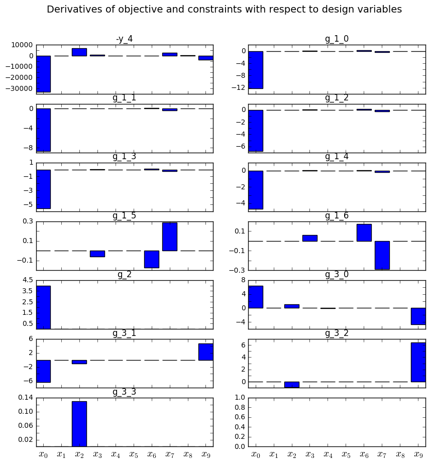
Gradient sensitivity on the Sobieski use case for the MDF formulation

\(x_0\) (wing-taper ratio) and \(x_2\) (Mach number) appear to be the most important for the gradient of the objective function.

The g_1_0 to g_1_4 are very similar, since they all quantify the stress in various sections. g_1_5 and g_1_6 correspond to the lower and upper bounds of the twist , therefore their sensitivities are opposite. g_2 is a function of only \(x_0\) ; \(x_0\) is the only variable that influences its gradient.