Self-Organizing Maps¶

Preliminaries: instantiation and execution of the MDO scenario¶

Let’s start with the following code lines which instantiate and execute the MDOScenario :

from gemseo.api import create_discipline, create_scenario

formulation = 'MDF'

disciplines = create_discipline(["SobieskiPropulsion", "SobieskiAerodynamics",
                                 "SobieskiMission", "SobieskiStructure"])

scenario = create_scenario(disciplines,
                           formulation=formulation,
                           objective_name="y_4",
                           maximize_objective=True,
                           design_space="design_space.txt")

scenario.set_differentiation_method("user")

algo_options = {'max_iter': 10, 'algo': "NLOPT_COBYLA"}
for constraint in ["g_1","g_2","g_3"]:
    scenario.add_constraint(constraint, 'ineq')

scenario.execute(algo_options)

SOM¶

Description¶

The SOM post processing perform a Self Organizing Map clustering on optimization history. A SOM is a 2D representation of a design of experiments which requires dimensionality reduction since it may be in very high dimension.

Options of the plot method are the figure width and height, and the x- and y- number of cells in the SOM. It is also possible either to save the plot, to show the plot or both.

Options¶

annotate, Unknown - add label of neuron value to SOM plot
extension, str - file extension
file_path, str - the base paths of the files to export
height, Unknown - figure height
n_x, int - x-size
n_y, int - y-size
save, bool - if True, exports plot to pdf
show, bool - if True, displays the plot windows
width, Unknown - figure width

Case of the MDF formulation¶

To plot the Self-Organizing Maps, use the API method execute_post() with the keyword “SOM”, the new dimension n_x and n_y and additional arguments concerning the type of display (file, screen, both):

scenario.post_process(“SOM”, save=False, n_x=4, n_y=4, show=True)

A SOM is built by using an unsupervised artificial neural network [KSH01]. A map of size n_x.n_y is generated, where n_x is the number of neurons in the \(x\) direction and n_y is the number of neurons in the \(y\) direction. The design space (whatever the dimension) is reduced to a 2D representation based on n_x.n_y neurons. Samples are clustered to a neuron when their design variables are close in terms of L2 norm. A neuron is always located at the same place on a map. Each neuron is colored according to the average value for a given criterion. This helps to qualitatively analyze if parts of the design space are good according to some criteria and not for others, and where compromises should be made. A white neuron has no sample associated with it: not enough evaluations were provided to train the SOM.

SOM provide a qualitative view of the objective function and the constraints, and of their relative behaviors.

Figure SOM example on the Sobieski problem illustrates a SOM on the Sobieski use case. The optimization method is a (costly) derivative free algorithm (NLOPT_COBYLA), since relevant are obtained at the cost of numerous evaluations of the functions. For more details, please read the paper by [KJO+06] on wing MDO post-processing using SOM.

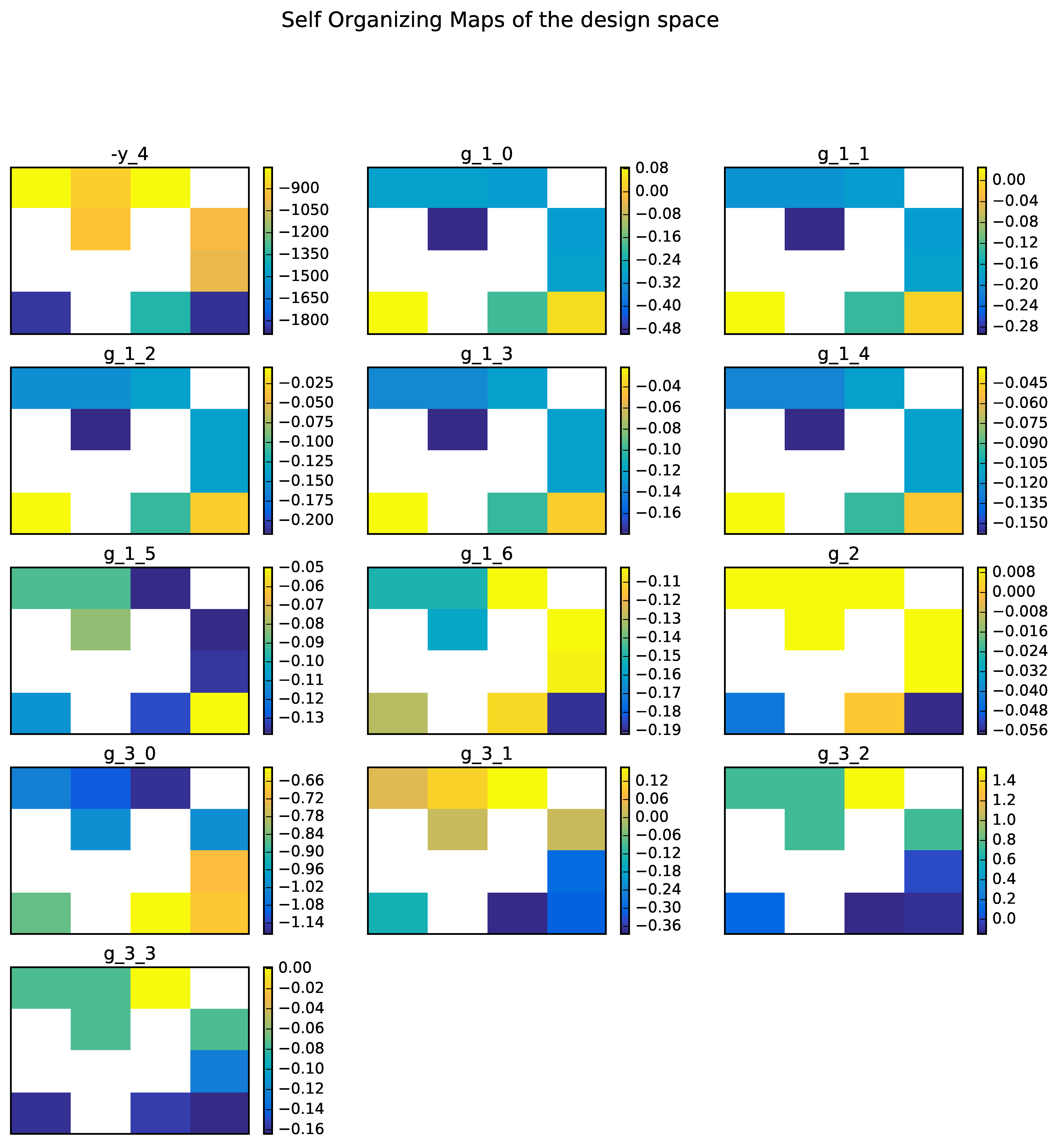
SOM example on the Sobieski problem¶

A DOE may also be a good way to produce SOM maps. In figure SOM example on the Sobieski problem with a 10 000 samples DOE is an example with 10000 points on the same test case. This produces more relevant SOM plots.

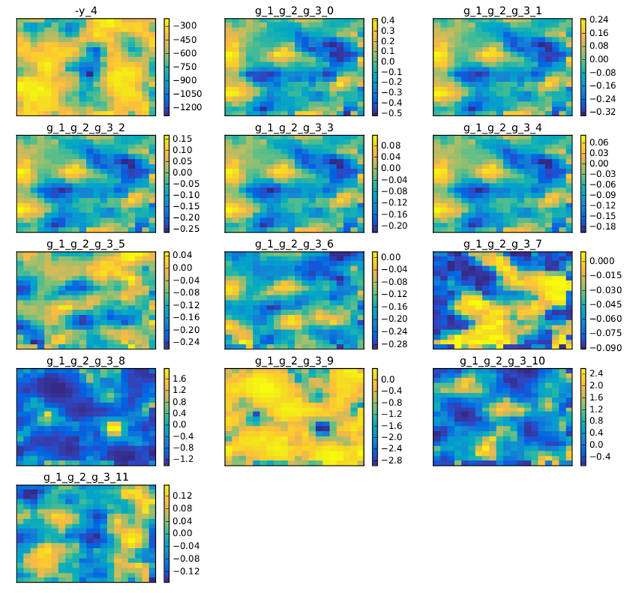
SOM example on the Sobieski problem with a 10 000 samples DOE¶