Tutorial: How to solve a MDO problem
This tutorial describes how to solve a MDO problem by means of GEMSEO. For that, we consider the Sellar problem.
Step 1 : Creation of disciplines
In order to solve the Sellar problem with GEMSEO, we need first to model this set of equations as a multidisciplinary problem.
For that, the problem is decomposed into three disciplines.
What defines a MDODiscipline
A discipline is a set of calculations that produces a set of vector outputs from a set of vector inputs, using either equations or an external software, or a workflow engine.
Programmatically speaking, in GEMSEO, a MDODiscipline is defined by three elements :
the input grammar : the set of rules that defines valid input data,
the output grammar : the set of rules that defines valid output data,
the method to compute the output data from the input data, here the
MDODiscipline._run()method.
The disciplines are all subclasses of MDODiscipline, from which they must inherit.
See also
The grammar is a very powerful and key concept. There are multiple ways of creating grammars in GEMSEO. The preferred one for integrating simulation processes is the use of a JSON schema, but is not detailed here for the sake of simplicity. For more explanations about grammars, see Interfacing simulation software.
Warning
All the inputs and outputs names of the disciplines in a scenario shall be consistent.
GEMSEO assumes that the data are tagged by their names with a global convention in the whole process.
What two disciplines call “X” shall be the same “X”. The coupling variables for instance, are detected thanks to these conventions.
1.1. Define the input and output grammars of the discipline
We create a class for each discipline inheriting from MDODiscipline.
After having called the superconstructor MDODiscipline.__init__(),
we complete the constructor of the new discipline by declaring the Sellar discipline input data names MDODiscipline.input_grammar and discipline output data names MDODiscipline.output_grammar in a straightforward way with
JSONGrammar.initialize_from_data_names() .
Warning
These inputs and outputs shall be numpy arrays of numbers. The grammars will check this at each execution and prevent any discipline from running with invalid data, or raise an error if outputs are invalid, which happens sometimes with simulation software…
For example, in the case of Sellar 1, we build:
from gemseo.core.discipline import MDODiscipline
from numpy import array, ones

class Sellar1(MDODiscipline):

    def __init__(self, residual_form=False):
        super(Sellar1, self).__init__()
        self.input_grammar.initialize_from_data_names(['x_local', 'x_shared', 'y_1'])
        self.output_grammar.initialize_from_data_names(['y_0'])
See also
An alternative way to declare the inputs and outputs is the usage of JSON schema, see Interfacing simulation software. This gives more control on the type of data that are considered valid inputs and outputs. In our case, it would look like this for the input declaration:
{
"name": "Sellar1_input",
"required": ["x_local","x_shared","y_0","y_1"],
"properties": {
    "x_local": {
        "items": {
            "type": "number"
        },
        "type": "array"
    },
    "x_shared": {
        "items": {
            "type": "number"
        },
        "type": "array"
    },
    "y_1": {
        "items": {
            "type": "number"
        },
        "type": "array"
    }
},
"$schema": "http://json-schema.org/draft-04/schema",
"type": "object",
}
1.2. Define the execution of the discipline
Once the inputs and outputs have been declared in the constructor of the discipline,
the abstract MDODiscipline._run() method of MDODiscipline shall be overloaded by
the discipline to define how outputs are computed from inputs.
See also
The method is protected (starts with “_”) because it shall not be called from outside the discipline.
External calls that trigger the discipline execution use the MDODiscipline.execute() public method from the base class,
which provides additional services before and after calling MDODiscipline._run(). These services, such as data checks by the grammars,
are provided by GEMSEO and the integrator of the discipline does not need to implement them.
First, the data values shall be retrieved. For each input declared in the input grammar, GEMSEO will pass the values as arrays to the MDODiscipline during the execution of the process.
There are different methods to get these values within the MDODiscipline._run() method of the discipline:
as a dictionary through the
MDODiscipline.get_input_data()method, which are also already accessible in theMDODiscipline.local_dataattribute of theMDODisciplineor here as a list of values using
MDODiscipline.get_inputs_by_name()with the data names passed as a list.
Tip
The list of all inputs names can also be retrieved using MDODiscipline.get_input_data_names():
sellar1 = Sellar1()
print(sellar1.get_input_data_names())
# ['x_shared', 'y_1', 'x_local']
Then, the computed outputs shall be stored in the MDODiscipline.local_data:
def _run(self):
    x_local, x_shared, y_1 = self.get_inputs_by_name(['x_local', 'x_shared', 'y_1'])
    self.local_data['y_0'] = array([x_shared[0] ** 2 + x_shared[1] + x_local[0] - 0.2 * y_1[0]])
The MDODiscipline.store_local_data() method can also be used to this aim:
def _run(self):
    x_local, x_shared, y_1 = self.get_inputs_by_name(['x_local', 'x_shared', 'y_1'])
    y_0 = array([x_shared[0] ** 2 + x_shared[1] + x_local[0] - 0.2 * y_1[0]])
    self.store_local_data(y_0=y_0)
The other Sellar MDODiscipline are created in a similar way.
1.3. How to define derivatives (optional)
The MDODiscipline may also provide the derivatives of their outputs with respect to their inputs, i.e. their Jacobians.
This is useful for gradient-based optimization or Multi Disciplinary Analyses based on the Newton method.
For a vector of inputs \(x\) and a vector of outputs \(y\), the Jacobian of the discipline is
\(\frac{\partial y}{\partial x}\).
The discipline shall provide a method to compute the Jacobian for a given set of inputs.
This is made by overloading the abstract MDODiscipline._compute_jacobian() method of MDODiscipline.
The discipline may have multiple inputs and multiple outputs. To store the multiple Jacobian matrices associated to all the inputs and outputs,
GEMSEO uses a dictionary of dictionaries structure. This data structure is sparse and makes easy the access and the iteration over the elements
of the Jacobian.
Here is an example of a jacobian definition for the Sellar1 discipline.
The method MDODiscipline._init_jacobian() fills the dict of dict structure
with dense null matrices of the right sizes. Note that all Jacobians must be 2D matrices, which avoids
ambiguity.
from numpy import atleast_2d

def _compute_jacobian(self, inputs=None, outputs=None):
    """
    Computes the jacobian

    :param inputs: linearization should be performed with respect
        to inputs list. If None, linearization should
        be performed wrt all inputs (Default value = None)
    :param outputs: linearization should be performed on outputs list.
        If None, linearization should be performed
        on all outputs (Default value = None)
    """
    # Initialize all matrices to zeros
    self._init_jacobian(with_zeros=True)
    x_local, x_shared, y_1 = self.get_inputs_by_name(['x_local', 'x_shared', 'y_1'])

    inv_denom = 1. / (self.compute_y_0(x_local, x_shared, y_1))
    self.jac['y_0'] = {}
    self.jac['y_0']['x_local'] = atleast_2d(array([0.5 * inv_denom]))
    self.jac['y_0']['x_shared'] = atleast_2d(array(
        [x_shared[0] * inv_denom, 0.5 * inv_denom]))
    self.jac['y_0']['y_1'] = atleast_2d(array([-0.1 * inv_denom]))
Synthetic Python code
In summary, here is the Python code for the three disciplines of the Sellar.
from math import exp, sqrt
from gemseo.core.discipline import MDODiscipline

class Sellar1(MDODiscipline):

    def __init__(self, residual_form=False):
        super(Sellar1, self).__init__()
        self.input_grammar.initialize_from_data_names(['x_local', 'x_shared', 'y_1'])
        self.output_grammar.initialize_from_data_names(['y_0'])

    def _run(self):
        x_local, x_shared, y_1 = self.get_inputs_by_name(['x_local', 'x_shared', 'y_1'])
        self.local_data['y_0'] = array([x_shared[0] ** 2 + x_shared[1] + x_local[0] - 0.2 * y_1[0]])

    def _compute_jacobian(self, inputs=None, outputs=None):
        self._init_jacobian(inputs, outputs, with_zeros=True)
        x_local, x_shared, y_1 = self.get_inputs_by_name(
            ['x_local', 'x_shared', 'y_1'])
        inv_denom = 1. / (self.compute_y_0(x_local, x_shared, y_1))
        self.jac['y_0'] = {}
        self.jac['y_0']['x_local'] = atleast_2d(array([0.5 * inv_denom]))
        self.jac['y_0']['x_shared'] = atleast_2d(array(
            [x_shared[0] * inv_denom, 0.5 * inv_denom]))
        self.jac['y_0']['y_1'] = atleast_2d(array([-0.1 * inv_denom]))

class Sellar2(MDODiscipline):

    def __init__(self, residual_form=False):
        super(Sellar2, self).__init__()
        self.input_grammar.initialize_from_data_names(['x_shared', 'y_0'])
        self.output_grammar.initialize_from_data_names(['y_1'])

    def _run(self):
        x_shared, y_0 = self.get_inputs_by_name(['x_shared', 'y_0'])
        self.local_data['y_1'] = array([sqrt(y_0) + x_shared[0] + x_shared[1]])

    def _compute_jacobian(self, inputs=None, outputs=None):
        self._init_jacobian(inputs, outputs, with_zeros=True)
        y_0 = self.get_inputs_by_name('y_0')
        self.jac['y_1'] = {}
        self.jac['y_1']['x_local'] = zeros((1, 1))
        self.jac['y_1']['x_shared'] = ones((1, 2))
        if y_0[0] < 0.:
            self.jac['y_1']['y_0'] = -ones((1, 1))
        elif y_0[0] == 0.:
            self.jac['y_1']['y_0'] = zeros((1, 1))
        else:
            self.jac['y_1']['y_0'] = ones((1, 1))

class SellarSystem(MDODiscipline):

    def __init__(self):
        super(SellarSystem, self).__init__()
        self.input_grammar.initialize_from_data_names(['x_local', 'x_shared', 'y_0', 'y_1'])
        self.output_grammar.initialize_from_data_names(['obj', 'c_1', 'c_2'])

    def _run(self):
        x_local, x_shared, y_0, y_1 = self.get_inputs_by_name(['x_local', 'x_shared', 'y_0', 'y_1'])
        self.local_data['obj'] = array([x_local[0] ** 2 + x_shared[1] + y_0[0] ** 2 + exp(-y_1[0])])
        self.local_data['c_1'] = array([1. - y_0[0] / 3.16])
        self.local_data['c_2'] = array([y_1[0] / 24. - 1.])

    def _compute_jacobian(self, inputs=None, outputs=None):
        self._init_jacobian(inputs, outputs, with_zeros=True)
        x_local, _, y_0, y_1 = self.get_inputs_by_name(
            ['x_local', 'x_shared', 'y_0', 'y_1'])
        self.jac['c_1']['y_0'] = atleast_2d(array([-2. * y_0]))
        self.jac['c_2']['y_1'] = ones((1, 1))
        self.jac['obj']['x_local'] = atleast_2d(array([2. * x_local[0]]))
        self.jac['obj']['x_shared'] = atleast_2d(array([0., 1.]))
        self.jac['obj']['y_0'] = atleast_2d(array([2. * y_0[0]]))
        self.jac['obj']['y_1'] = atleast_2d(array([-exp(-y_1[0])]))
Shortcut
The classes Sellar1, Sellar2 and SellarSystem are available in the directory gemseo/problems/sellar. Consequently, you just need to import them and use it!
from gemseo.problems.sellar.sellar import Sellar1, Sellar2, SellarSystem

disciplines = [Sellar1(), Sellar2(), SellarSystem()]
A more simplest alternative consists of using the create_discipline() API function:
from gemseo.api import create_discipline

disciplines = create_discipline(['Sellar1', 'Sellar2', 'SellarSystem'])
Going further
For more information about the connection of software with GEMSEO, in particular the concepts and what goes on under the hood, please see Interfacing simulation software.
Step 2: Creation and execution of the MDO scenario
From the MDODiscipline, we build the scenario.
The scenario is responsible for the creation and execution of the whole process.
It will:
build an optimization problem using a MDO formulation,
connect it to a selected optimization algorithm,
solve the optimization problems
post-process the results.
For that, we use the class MDOScenario which is defined by different MDODiscipline and a common DesignSpace
2.1. Create the MDODiscipline
To instantiate the MDOScenario, we need first the MDODiscipline instances.
from gemseo.api import create_discipline

disciplines = create_discipline(['Sellar1', 'Sellar2', 'SellarSystem'])
2.2. Create the DesignSpace
Then, by means of the API function gemseo.api.create_design_space(), we build the DesignSpace, which defines the design variables, with their bounds and values:
from numpy import ones, array
from gemseo.api import create_design_space

design_space = create_design_space()
design_space.add_variable('x_local', 1, l_b=0., u_b=10., value=ones(1))
design_space.add_variable('x_shared', 2, l_b=(-10, 0.), u_b=(10., 10.), value=array([4., 3.]))
design_space.add_variable('y_0', 1, l_b=-100., u_b=100., value=ones(1))
design_space.add_variable('y_1', 1, l_b=-100., u_b=100., value=ones(1))
Warning
Here, we also add the coupling variables in the DesignSpace, even if we are going to use a MDF formulation, which computes the coupling using an Multi Disciplinary Analyses:
The formulation will by itself remove the coupling variables from the optimization unknowns, but will use the values as default values for the inputs of the
MDODiscipline.This will also be convenient when we will switch to the IDF, which uses the coupling variables as optimization unknowns.
Alternatively, one can perform MDF without coupling variables in the DesignSpace, but set the default values of the inputs using the MDODiscipline.default_inputs
attribute to the three disciplines:
discipline[0].default_inputs = {'y_1': ones(1)}
discipline[1].default_inputs = {'y_0': ones(1)}
discipline[2].default_inputs = {'y_0': ones(1), 'y_1': ones(1)}
2.3. Create the MDOScenario
Then, by means of the API function gemseo.api.create_scenario(),
we create the process which is a MDOScenario.
The scenario delegates the creation of an OptimizationProblem to the MDOFormulation.
We choose the MDF formulation, which solves a coupling problem (Multi Disciplinary Analyses) at each iteration to compute the coupling variables,
here the \(y_0\) and \(y_1\) variables, from both \(x_{local}\) and \(x_{shared}\) variables.
To be executable, the scenario needs at least an objective function. The constraints being optional.
The name of the objective function shall be one of the outputs of the disciplines. Here, the SellarSystem discipline
outputs “obj”, “c_1”, and “c_2”, which are declared as, respectively, the objective function and inequality constraints.
from gemseo.api import create_scenario

scenario = create_scenario(disciplines, 'MDF', 'obj', design_space)
Users may add constraints to the optimization problem.
scenario.add_constraint('c_1', 'ineq')
scenario.add_constraint('c_2', 'ineq')
The execution of the process is triggered through the resolution of the optimization problem
by an optimizer. The name of the optimizer and its options are given to the scenario as input data in a Python dictionary.
Here the SLSQP algorithm is a gradient-based optimization algorithm.
The disciplines that we integrated provide no analytical derivatives,
so we need first to tell the scenario to use finite differences to compute the derivatives using Scenario.set_differentiation_method().
scenario.set_differentiation_method('finite_differences', 1e-6)
2.4. Solve the OptimizationProblem
Then, we can run the scenario by calling the MDODiscipline.execute() method of the scenario.
scenario.execute(input_data={'max_iter': 10, 'algo': 'SLSQP'})
The logging message provides substantial information about the process setup, execution and results.
*** Start MDO Scenario execution ***
MDOScenario:
Disciplines: Sellar1 Sellar2 SellarSystem
MDOFormulation: MDF
Algorithm: SLSQP

Optimization problem:
      Minimize: obj(x_local, x_shared)
With respect to:
    x_local, x_shared
Subject to constraints:
c_1(x_local, x_shared) <= 0
c_2(x_local, x_shared) <= 0
Design Space:
+-------------+-------------+-------+-------------+-------+
| name        | lower_bound | value | upper_bound | type  |
+-------------+-------------+-------+-------------+-------+
| x_local     |      0      |   1   |      10     | float |
| x_shared    |     -10     |   4   |      10     | float |
| x_shared    |      0      |   3   |      10     | float |
+-------------+-------------+-------+-------------+-------+
Optimization: |          | 0/10   0% [elapsed: 00:00 left: ?, ? iters/sec]
Optimization: |████      | 4/10  40% [elapsed: 00:00 left: 00:00, 35.47 iters/sec obj: 28.94 ]
Optimization: |███████   | 7/10  70% [elapsed: 00:00 left: 00:00, 29.73 iters/sec obj: 10.50 ]
Optimization: |█████████ | 9/10  90% [elapsed: 00:00 left: 00:00, 25.33 iters/sec obj: 10.01 ]
Optimization result:
Objective value = 10.0089939499
The result is feasible.
Status: 0
Optimizer message: Optimization terminated successfully.
Number of calls to the objective function by the optimizer: 9

Design Space:
+-------------+-------------+-----------------------+-------------+-------+
| name        | lower_bound |         value         | upper_bound | type  |
+-------------+-------------+-----------------------+-------------+-------+
| x_local     |      0      |           0           |      10     | float |
| x_shared    |     -10     |    1.97763896744452   |      10     | float |
| x_shared    |      0      | 9.872903658415667e-11 |      10     | float |
+-------------+-------------+-----------------------+-------------+-------+
*** MDO Scenario run terminated in 0:00:00.362954 ***
Step 3: Post-processing of the results
Finally, we generate plots of the optimization history: the design variables, the objective function and the constraints values. For a complete description of available post-processing, see How to deal with post-processing.
scenario.post_process("OptHistoryView", save=True)
This generates PDF plots:

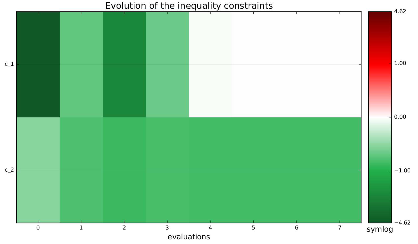
The constraints values history

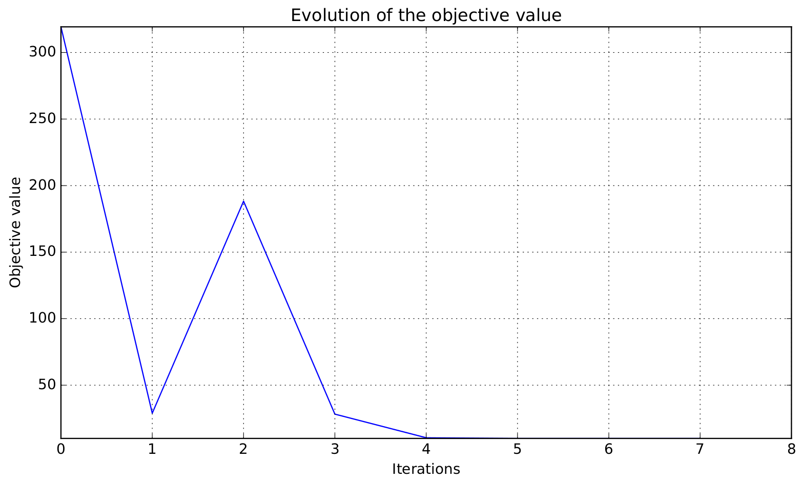
The objective function values history

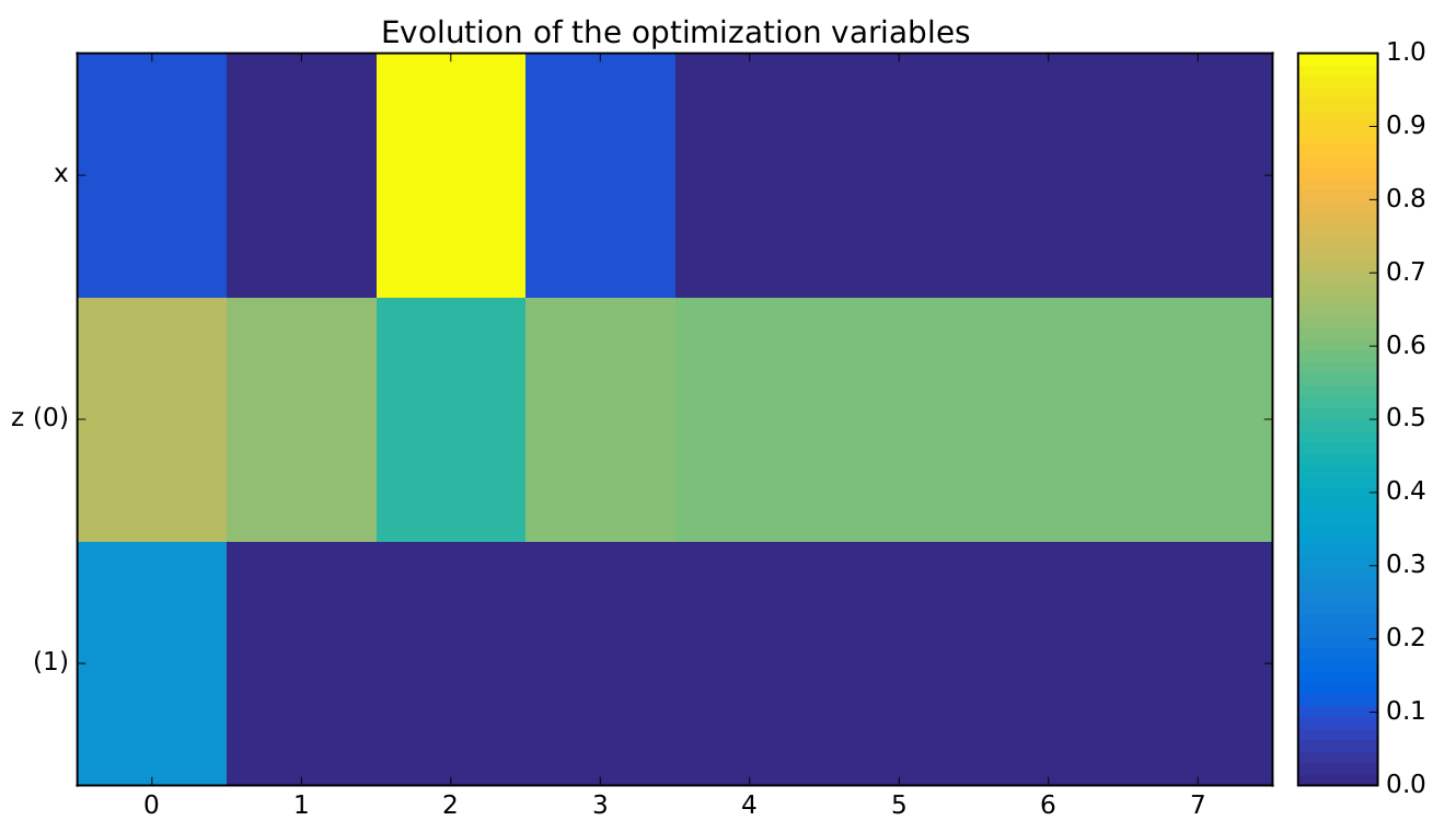
The design variables values history
Synthetic Python code
from numpy import array, ones
from gemseo.api import create_discipline, create_design_space, create_scenario

# Step 1: create the disciplines
disciplines = create_discipline(['Sellar1', 'Sellar2', 'SellarSystem'])
# Step 2: create the design space
design_space = create_design_space()
design_space.add_variable('x_local', 1, l_b=0., u_b=10., value=ones(1))
design_space.add_variable('x_shared', 2, l_b=(-10, 0.), u_b=(10., 10.), value=array([4., 3.]))
design_space.add_variable('y_0', 1, l_b=-100., u_b=100., value=ones(1))
design_space.add_variable('y_1', 1, l_b=-100., u_b=100., value=ones(1))
# Step 3: create and solve the MDO scenario
scenario = create_scenario(disciplines, 'MDF', objective_name='obj', design_space=design_space)
scenario.set_differentiation_method('finite_differences', 1e-6)
scenario.default_inputs = {'max_iter': 10, 'algo': 'SLSQP'})
scenario.execute()
# Step 4: analyze the results
scenario.post_process("OptHistoryView", save=True)
Easily switching between MDO formulations
One of the main interests of GEMSEO is the ability to switch between MDO formulations very easily. Basically you just need to change the name of the formulation in the script.
Tip
Available formulations can obtained through the API function
gemseo.api.get_available_formulations(). The following Python lines
from gemseo.api import get_available_formulations

print(get_available_formulations())
give:
['IDF', 'BiLevel', 'MDF', 'DisciplinaryOpt']
Here, we are going to try the IDF formulation, which is another classical MDO formulation along with MDF:
scenario = MDOScenario(disciplines, 'IDF', objective_name='obj', design_space=design_space)
In IDF, all disciplines are executed independently, and the coupling variables are unknown from the optimizer.
In fact the optimizer will solve the coupling problem simultaneously with the optimization problem by adding so-called consistency constraints (see MDO formulations).
The IDF class will create the consistency equality constraints for you.
The logging message shows that the generated optimization problem is different, while the disciplines remain the same. One can note the consistency equality constraints, used to solve the coupling problem. The design space now contains the coupling variables.
*** Start MDO Scenario execution ***
MDOScenario:
Disciplines: Sellar1 Sellar2 SellarSystem
MDOFormulation: IDF
Algorithm: SLSQP

Optimization problem:
      Minimize: obj(x_loca, x_shared, y_0, y_1)
With respect to:
    x_local, x_shared, y_0, y_1
Subject to constraints:
y_0(x_local, x_shared, y_1) = y_0(x_local, x_shared, y_1) - y_0 = 0
y_1(x_shared, y_0) = y_1(x_shared, y_0) - y_1 = 0
c_1(x_local, x_shared, y_0, y_1) <= 0
c_2(x_local, x_shared, y_0, y_1) <= 0
Design Space:
+-------------+-------------+-------+-------------+-------+
| name        | lower_bound | value | upper_bound | type  |
+-------------+-------------+-------+-------------+-------+
| x_local     |      0      |   1   |      10     | float |
| x_shared    |     -10     |   4   |      10     | float |
| x_shared    |      0      |   3   |      10     | float |
| y_0         |     -100    |   1   |     100     | float |
| y_1         |     -100    |   1   |     100     | float |
+-------------+-------------+-------+-------------+-------+
The results are similar, and the execution duration is 4 times shorter than in the previous case. Indeed, the IDF formulation does not need to solve an Multi Disciplinary Analyses at each step, and is often more efficient in low dimension.
Optimization: |          | 0/10   0% [elapsed: 00:00 left: ?, ? iters/sec]
Optimization: |███████   | 7/10  70% [elapsed: 00:00 left: 00:00, 101.65 iters/sec]
Optimization result:
Objective value = 10.0089731042
The result is feasible.
Status: 0
Optimizer message: Optimization terminated successfully.
Number of calls to the objective function by the optimizer: 7

Design Space:
+------+-------------+-----------------------+-------------+-------+
| name | lower_bound |         value         | upper_bound | type  |
+------+-------------+-----------------------+-------------+-------+
| x    |      0      | 4.258931532094556e-11 |      10     | float |
| z    |     -10     |   1.978530433409389   |      10     | float |
| z    |      0      |  2.2557630473285e-11  |      10     | float |
| y_0  |     -100    |   3.160000000019167   |     100     | float |
| y_1  |     -100    |   3.756169316899445   |     100     | float |
+------+-------------+-----------------------+-------------+-------+
*** MDO Scenario run terminated in 0:00:00.077177 ***
