Morris analysis

import pprint

from matplotlib import pyplot as plt
from numpy import pi

from gemseo.algos.parameter_space import ParameterSpace
from gemseo.api import create_discipline
from gemseo.uncertainty.sensitivity.morris.analysis import MorrisAnalysis

In this example, we consider a function from \([-\pi,\pi]^3\) to \(\mathbb{R}^3\):

\[(y_1,y_2)=\left(f(x_1,x_2,x_3),f(x_2,x_1,x_3)\right)\]

where \(f(a,b,c)=\sin(a)+7\sin(b)^2+0.1*c^4\sin(a)\) is the Ishigami function:

expressions = {
    "y1": "sin(x1)+7*sin(x2)**2+0.1*x3**4*sin(x1)",
    "y2": "sin(x2)+7*sin(x1)**2+0.1*x3**4*sin(x2)",
}
discipline = create_discipline(
    "AnalyticDiscipline", expressions_dict=expressions, name="Ishigami2"
)

Then, we consider the case where the deterministic variables \(x_1\), \(x_2\) and \(x_3\) are replaced with the uncertain variables \(X_1\), \(X_2\) and \(X_3\). The latter are independent and identically distributed according to an uniform distribution between \(-\pi\) and \(\pi\):

space = ParameterSpace()
for variable in ["x1", "x2", "x3"]:
    space.add_random_variable(
        variable, "OTUniformDistribution", minimum=-pi, maximum=pi
    )

From that, we would like to carry out a sensitivity analysis with the random outputs \(Y_1=f(X_1,X_2,X_3)\) and \(Y_2=f(X_2,X_1,X_3)\). For that, we can compute the correlation coefficients from a MorrisAnalysis:

morris = MorrisAnalysis(discipline, space, 10)
morris.compute_indices()

Out:

{'mu': {'y1': [{'x1': array([-0.36000398]), 'x2': array([0.77781853]), 'x3': array([-0.70990541])}], 'y2': [{'x1': array([-0.29766709]), 'x2': array([0.26848457]), 'x3': array([-0.7755748])}]}, 'mu_star': {'y1': [{'x1': array([0.67947346]), 'x2': array([0.88906579]), 'x3': array([0.72694219])}], 'y2': [{'x1': array([1.33011973]), 'x2': array([0.38907897]), 'x3': array([1.00221431])}]}, 'sigma': {'y1': [{'x1': array([0.98724949]), 'x2': array([0.79064599]), 'x3': array([0.8074493])}], 'y2': [{'x1': array([1.46392293]), 'x2': array([0.39387241]), 'x3': array([1.38465263])}]}}

The resulting indices are the empirical means and the standard deviations of the absolute output variations due to input changes.

pprint.pprint(morris.indices)

Out:

{'mu': {'y1': [{'x1': array([-0.36000398]),
                'x2': array([0.77781853]),
                'x3': array([-0.70990541])}],
        'y2': [{'x1': array([-0.29766709]),
                'x2': array([0.26848457]),
                'x3': array([-0.7755748])}]},
 'mu_star': {'y1': [{'x1': array([0.67947346]),
                     'x2': array([0.88906579]),
                     'x3': array([0.72694219])}],
             'y2': [{'x1': array([1.33011973]),
                     'x2': array([0.38907897]),
                     'x3': array([1.00221431])}]},
 'sigma': {'y1': [{'x1': array([0.98724949]),
                   'x2': array([0.79064599]),
                   'x3': array([0.8074493])}],
           'y2': [{'x1': array([1.46392293]),
                   'x2': array([0.39387241]),
                   'x3': array([1.38465263])}]}}

The main indices corresponds to the Spearman correlation indices (this main method can be changed with MorrisAnalysis.main_method):

pprint.pprint(morris.main_indices)

Out:

{'y1': [{'x1': array([0.67947346]),
         'x2': array([0.88906579]),
         'x3': array([0.72694219])}],
 'y2': [{'x1': array([1.33011973]),
         'x2': array([0.38907897]),
         'x3': array([1.00221431])}]}

We can also sort the input parameters by decreasing order of influence and observe that this ranking is not the same for both outputs:

print(morris.sort_parameters("y1"))
print(morris.sort_parameters("y2"))

Out:

['x2', 'x3', 'x1']
['x1', 'x3', 'x2']

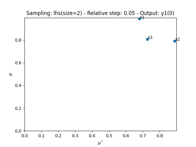
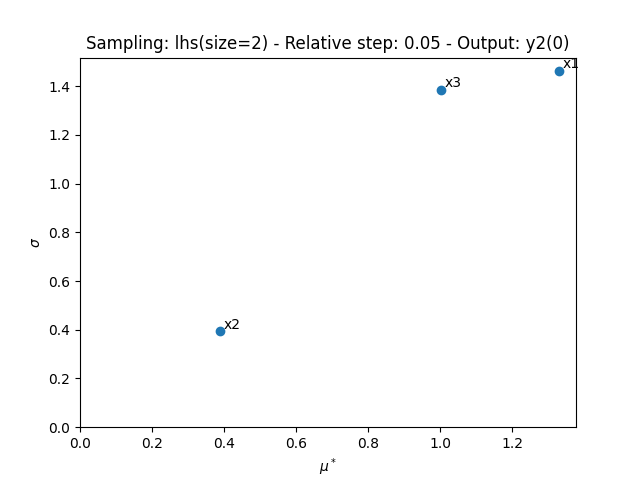
Lastly, we can use the method MorrisAnalysis.plot() to visualize the different series of indices:

morris.plot("y1", save=False, show=False, lower_mu=0, lower_sigma=0)
morris.plot("y2", save=False, show=False, lower_mu=0, lower_sigma=0)
# Workaround for HTML rendering, instead of ``show=True``
plt.show()

• 
•