Scatter plot matrix¶

Preliminaries: instantiation and execution of the MDO scenario¶

Let’s start with the following code lines which instantiate and execute the MDOScenario :

from gemseo.api import create_discipline, create_scenario

formulation = 'MDF'

disciplines = create_discipline(["SobieskiPropulsion", "SobieskiAerodynamics",
                                 "SobieskiMission", "SobieskiStructure"])

scenario = create_scenario(disciplines,
                           formulation=formulation,
                           objective_name="y_4",
                           maximize_objective=True,
                           design_space="design_space.txt")

scenario.set_differentiation_method("user")

algo_options = {'max_iter': 10, 'algo': "SLSQP"}
for constraint in ["g_1","g_2","g_3"]:
    scenario.add_constraint(constraint, 'ineq')

scenario.execute(algo_options)

ScatterPlotMatrix¶

Description¶

The ScatterPlotMatrix post processing builds the scatter plot matrix among design variables, outputs functions and constraints.

The list of variable names has to be passed as arguments of the plot method. x- and y- figure sizes can be changed in option. It is possible either to save the plot, to show the plot or both.

Options¶

variables_list, list(str) - The function names or design variables to plot. If the list is empty, plot all design variables.
figsize_x, int - The size of the figure in the horizontal direction (inches).
figsize_y, int - The size of the figure in the vertical direction (inches).
show, bool - If True, display the plot windows.
save, bool - If True, export the plot to a file.
file_path, str - The base path of the files to export. Relative to the working directory.
extension, str - The file extension.

Case of the MDF formulation¶

To visualize the scatter plot matrix of the scenario, we use the execute_post() API method with the keyword "ScatterPlotMatrix" and additional arguments concerning the type of display (file, screen, both):

scenario.post_process("ScatterPlotMatrix", variables_list=["-y_4", "x_1", "g_2"], save=False, show=True, file_path="mdf")

In the figure Scatter Plot Matrix on the Sobieski use case for the MDF formulation, each non-diagonal block represents the samples according to the x- and y- coordinates names while the diagonal ones approximate the probability distributions of the variables, using a kernel-density estimator.

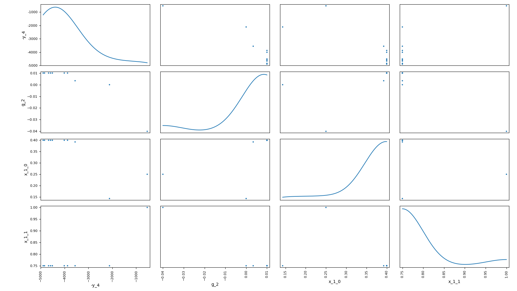
../../_images/mdf_scatter_plot_matrix.png — Scatter Plot Matrix on the Sobieski use case for the MDF formulation¶