Note
Click here to download the full example code
Mixture of experts
In this demo, we load a dataset (the Rosenbrock function in 2D) and apply a mixture of experts regression model to obtain an approximation.
from __future__ import division, unicode_literals

import matplotlib.pyplot as plt
from numpy import array, hstack, linspace, meshgrid, nonzero, sqrt, zeros

from gemseo.api import configure_logger, load_dataset
from gemseo.mlearning.api import create_regression_model
from gemseo.mlearning.transform.scaler.min_max_scaler import MinMaxScaler

configure_logger()
Out:
<RootLogger root (INFO)>
Dataset (Rosenbrock)
We here consider the Rosenbrock function with two inputs, on the interval \([-2, 2] \times [-2, 2]\).
Load dataset
A prebuilt dataset for the Rosenbrock function with two inputs is given as a dataset parametrization, based on a full factorial DOE of the input space with 100 points.
dataset = load_dataset("RosenbrockDataset", opt_naming=False)
Print information
Information about the dataset can easily be displayed by printing the dataset directly.
print(dataset)
Out:
Rosenbrock
   Number of samples: 100
   Number of variables: 2
   Variables names and sizes by group:
      inputs: x (2)
      outputs: rosen (1)
   Number of dimensions (total = 3) by group:
      inputs: 2
      outputs: 1
Show dataset
The dataset object can present the data in tabular form.
print(dataset.export_to_dataframe())
Out:
      inputs           outputs
           x             rosen
           0    1            0
0  -2.000000 -2.0  3609.000000
1  -1.555556 -2.0  1959.952599
2  -1.111111 -2.0  1050.699741
3  -0.666667 -2.0   600.308642
4  -0.222222 -2.0   421.490779
..       ...  ...          ...
95  0.222222  2.0   381.095717
96  0.666667  2.0   242.086420
97  1.111111  2.0    58.600975
98  1.555556  2.0    17.927907
99  2.000000  2.0   401.000000

[100 rows x 3 columns]
Mixture of experts (MoE)
In this section we load a mixture of experts regression model through the machine learning API, using clustering, classification and regression models.
Mixture of experts model
We construct the MoE model using the predefined parameters, and fit the model to the dataset through the learn() method.
model = create_regression_model(
    "MixtureOfExperts", dataset, transformer={"outputs": MinMaxScaler()}
)
model.set_clusterer("KMeans", n_clusters=3)
model.set_classifier("KNNClassifier", n_neighbors=5)
model.set_regressor("GaussianProcessRegression")

model.learn()
Tests
Here, we test the mixture of experts method applied to two points: (1, 1), the global minimum, where the function is zero, and (-2, -2), an extreme point where the function has a high value (max on the domain). The classes are expected to be different at the two points.
input_value = {"x": array([1, 1])}
another_input_value = {"x": array([[1, 1], [-2, -2]])}

for value in [input_value, another_input_value]:
    print("Input value:", value)
    print("Class:", model.predict_class(value))
    print("Prediction:", model.predict(value))
    print("Local model predictions:")
    for cls in range(model.n_clusters):
        print("Local model {}: {}".format(cls, model.predict_local_model(value, cls)))
    print()
Out:
Input value: {'x': array([1, 1])}
Class: {'labels': array([0])}
Prediction: {'rosen': array([4.17031586])}
Local model predictions:
Local model 0: {'rosen': array([4.17031586])}
Local model 1: {'rosen': array([532.87624246])}
Local model 2: {'rosen': array([-46.32257302])}

Input value: {'x': array([[ 1,  1],
       [-2, -2]])}
Class: {'labels': array([[0],
       [2]])}
Prediction: {'rosen': array([[   4.17031586],
       [3608.99981798]])}
Local model predictions:
Local model 0: {'rosen': array([[  4.17031586],
       [409.41192877]])}
Local model 1: {'rosen': array([[ 532.87624246],
       [3514.58059484]])}
Local model 2: {'rosen': array([[ -46.32257302],
       [3608.99981798]])}
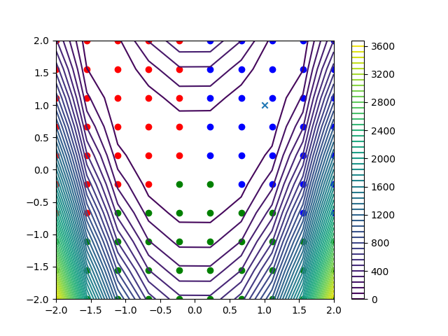
Plot clusters
Here, we plot the 10x10 = 100 Rosenbrock function data points, with colors representing the obtained clusters. The Rosenbrock function is represented by a contour plot in the background.
n_samples = dataset.n_samples
# Dataset is based on a DOE of 100=10^2 fullfact.
input_dim = int(sqrt(n_samples))
assert input_dim ** 2 == n_samples  # Check that n_samples is a square number

colors = ["b", "r", "g", "o", "y"]
inputs = dataset.get_data_by_group(dataset.INPUT_GROUP)
outputs = dataset.get_data_by_group(dataset.OUTPUT_GROUP)
x = inputs[:input_dim, 0]
y = inputs[:input_dim, 0]

Z = zeros((input_dim, input_dim))
for i in range(input_dim):
    Z[i, :] = outputs[input_dim * i : input_dim * (i + 1), 0]
fig = plt.figure()
cnt = plt.contour(x, y, Z, 50)
fig.colorbar(cnt)
for index in range(model.n_clusters):
    samples = nonzero(model.labels == index)[0]
    plt.scatter(inputs[samples, 0], inputs[samples, 1], color=colors[index])
plt.scatter(1, 1, marker="x")
plt.show()
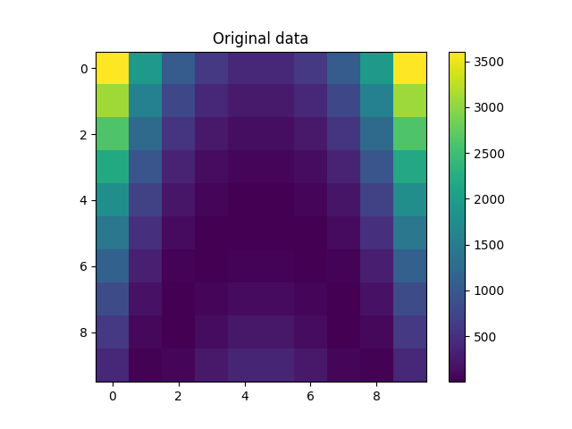
Plot data and predictions from final model
We construct a refined input space, and compute the model predictions.
refinement = 200
fine_x = linspace(x[0], x[-1], refinement)
fine_y = linspace(y[0], y[-1], refinement)
fine_x, fine_y = meshgrid(fine_x, fine_y)
fine_input = {"x": hstack([fine_x.flatten()[:, None], fine_y.flatten()[:, None]])}
fine_z = model.predict(fine_input)
# Reshape
fine_z = fine_z["rosen"].reshape((refinement, refinement))
plt.figure()
plt.imshow(Z)
plt.colorbar()
plt.title("Original data")
plt.show()
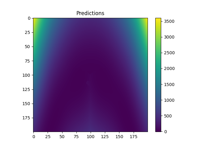
plt.figure()
plt.imshow(fine_z)
plt.colorbar()
plt.title("Predictions")
plt.show()
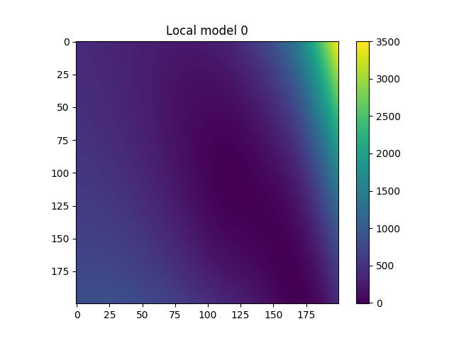
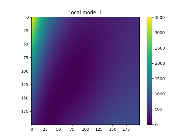
Plot local models
for i in range(model.n_clusters):
    plt.figure()
    plt.imshow(
        model.predict_local_model(fine_input, i)["rosen"].reshape(
            (refinement, refinement)
        )
    )
    plt.colorbar()
    plt.title("Local model {}".format(i))
    plt.show()

Total running time of the script: ( 0 minutes 3.047 seconds)