Note
Click here to download the full example code
Optimization History View
In this example, we illustrate the use of the OptHistoryView plot
on the Sobieski’s SSBJ problem.
from __future__ import division, unicode_literals

from matplotlib import pyplot as plt
Import
The first step is to import some functions from the API and a method to get the design space.
from gemseo.api import configure_logger, create_discipline, create_scenario
from gemseo.problems.sobieski.core import SobieskiProblem

configure_logger()
Out:
<RootLogger root (INFO)>
Description
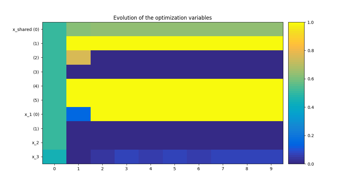
The OptHistoryView post-processing creates a series of plots:
The design variables history - This graph shows the normalized values of the design variables, the \(y\) axis is the index of the inputs in the vector; and the \(x\) axis represents the iterations.
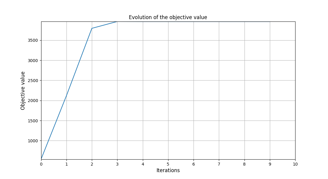
The objective function history - It shows the evolution of the objective value during the optimization.
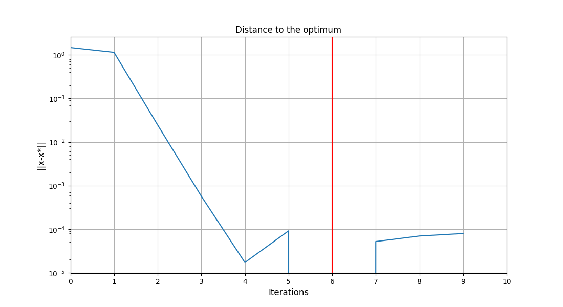
The distance to the best design variables - Plots the vector \(log( ||x-x^*|| )\) in log scale.
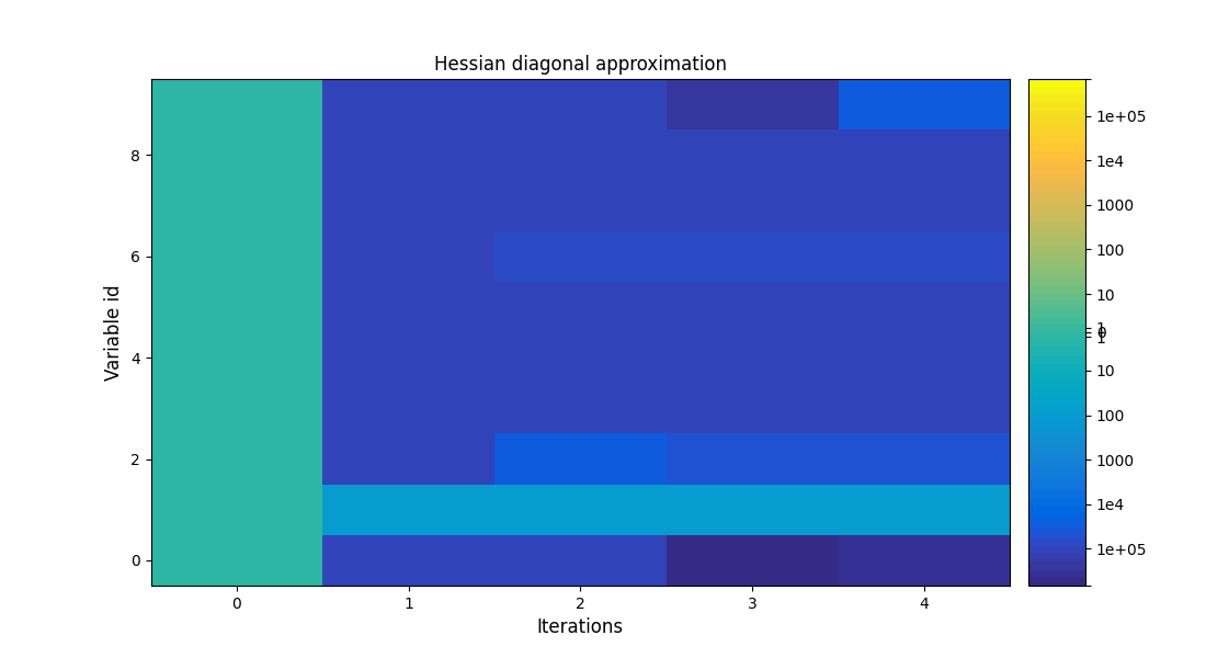
The history of the Hessian approximation of the objective - Plots an approximation of the second order derivatives of the objective function \(\frac{\partial^2 f(x)}{\partial x^2}\), which is a measure of the sensitivity of the function with respect to the design variables, and of the anisotropy of the problem (differences of curvatures in the design space).
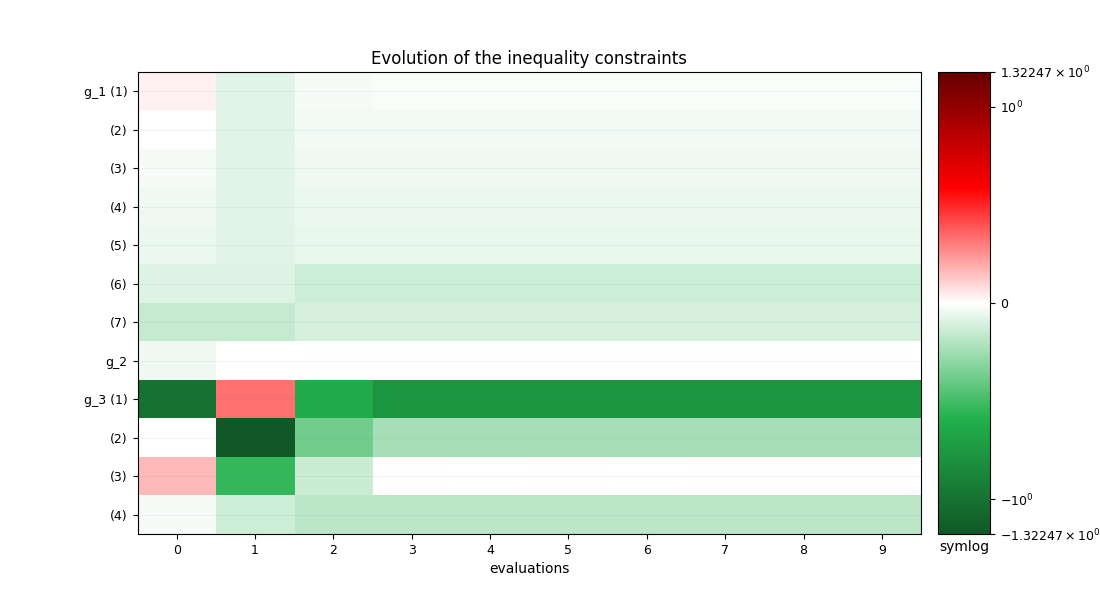
The inequality constraint history - Portrays the evolution of the values of the constraints. The inequality constraints must be non-positive, that is why the plot must be green or white for satisfied constraints (white = active, red = violated). For an IDF formulation, an additional plot is created to track the equality constraint history.
Create disciplines
At this point we instantiate the disciplines of Sobieski’s SSBJ problem: Propulsion, Aerodynamics, Structure and Mission
disciplines = create_discipline(
    [
        "SobieskiPropulsion",
        "SobieskiAerodynamics",
        "SobieskiStructure",
        "SobieskiMission",
    ]
)
Create design space
We also read the design space from the SobieskiProblem.
design_space = SobieskiProblem().read_design_space()
Create and execute scenario
The next step is to build an MDO scenario in order to maximize the range, encoded ‘y_4’, with respect to the design parameters, while satisfying the inequality constraints ‘g_1’, ‘g_2’ and ‘g_3’. We can use the MDF formulation, the SLSQP optimization algorithm and a maximum number of iterations equal to 100.
scenario = create_scenario(
    disciplines,
    formulation="MDF",
    objective_name="y_4",
    maximize_objective=True,
    design_space=design_space,
)
scenario.set_differentiation_method("user")
for constraint in ["g_1", "g_2", "g_3"]:
    scenario.add_constraint(constraint, "ineq")
scenario.execute({"algo": "SLSQP", "max_iter": 10})
Out:
    INFO - 14:42:16:
    INFO - 14:42:16: *** Start MDO Scenario execution ***
    INFO - 14:42:16: MDOScenario
    INFO - 14:42:16:    Disciplines: SobieskiPropulsion SobieskiAerodynamics SobieskiStructure SobieskiMission
    INFO - 14:42:16:    MDOFormulation: MDF
    INFO - 14:42:16:    Algorithm: SLSQP
    INFO - 14:42:16: Optimization problem:
    INFO - 14:42:16:    Minimize: -y_4(x_shared, x_1, x_2, x_3)
    INFO - 14:42:16:    With respect to: x_shared, x_1, x_2, x_3
    INFO - 14:42:16:    Subject to constraints:
    INFO - 14:42:16:       g_1(x_shared, x_1, x_2, x_3) <= 0.0
    INFO - 14:42:16:       g_2(x_shared, x_1, x_2, x_3) <= 0.0
    INFO - 14:42:16:       g_3(x_shared, x_1, x_2, x_3) <= 0.0
    INFO - 14:42:16: Design space:
    INFO - 14:42:16: +----------+-------------+-------+-------------+-------+
    INFO - 14:42:16: | name     | lower_bound | value | upper_bound | type  |
    INFO - 14:42:16: +----------+-------------+-------+-------------+-------+
    INFO - 14:42:16: | x_shared |     0.01    |  0.05 |     0.09    | float |
    INFO - 14:42:16: | x_shared |    30000    | 45000 |    60000    | float |
    INFO - 14:42:16: | x_shared |     1.4     |  1.6  |     1.8     | float |
    INFO - 14:42:16: | x_shared |     2.5     |  5.5  |     8.5     | float |
    INFO - 14:42:16: | x_shared |      40     |   55  |      70     | float |
    INFO - 14:42:16: | x_shared |     500     |  1000 |     1500    | float |
    INFO - 14:42:16: | x_1      |     0.1     |  0.25 |     0.4     | float |
    INFO - 14:42:16: | x_1      |     0.75    |   1   |     1.25    | float |
    INFO - 14:42:16: | x_2      |     0.75    |   1   |     1.25    | float |
    INFO - 14:42:16: | x_3      |     0.1     |  0.5  |      1      | float |
    INFO - 14:42:16: +----------+-------------+-------+-------------+-------+
    INFO - 14:42:16: Optimization:   0%|          | 0/10 [00:00<?, ?it]
/home/docs/checkouts/readthedocs.org/user_builds/gemseo/conda/3.2.2/lib/python3.8/site-packages/scipy/sparse/linalg/dsolve/linsolve.py:407: SparseEfficiencyWarning: splu requires CSC matrix format
  warn('splu requires CSC matrix format', SparseEfficiencyWarning)
    INFO - 14:42:16: Optimization:  20%|██        | 2/10 [00:00<00:00, 53.32 it/sec, obj=2.12e+3]
    INFO - 14:42:17: Optimization:  40%|████      | 4/10 [00:00<00:00, 21.38 it/sec, obj=3.97e+3]
    INFO - 14:42:17: Optimization:  50%|█████     | 5/10 [00:00<00:00, 16.68 it/sec, obj=3.96e+3]
    INFO - 14:42:17: Optimization:  60%|██████    | 6/10 [00:00<00:00, 13.64 it/sec, obj=3.96e+3]
    INFO - 14:42:17: Optimization:  70%|███████   | 7/10 [00:00<00:00, 11.54 it/sec, obj=3.96e+3]
    INFO - 14:42:17: Optimization:  90%|█████████ | 9/10 [00:01<00:00,  9.84 it/sec, obj=3.96e+3]
    INFO - 14:42:17: Optimization: 100%|██████████| 10/10 [00:01<00:00,  9.15 it/sec, obj=3.96e+3]
    INFO - 14:42:17: Optimization result:
    INFO - 14:42:17: Objective value = 3963.595455433326
    INFO - 14:42:17: The result is feasible.
    INFO - 14:42:17: Status: None
    INFO - 14:42:17: Optimizer message: Maximum number of iterations reached. GEMSEO Stopped the driver
    INFO - 14:42:17: Number of calls to the objective function by the optimizer: 12
    INFO - 14:42:17: Constraints values:
    INFO - 14:42:17:    g_1 = [-0.01814919 -0.03340982 -0.04429875 -0.05187486 -0.05736009 -0.13720854
    INFO - 14:42:17:  -0.10279146]
    INFO - 14:42:17:    g_2 = 3.236261671801799e-05
    INFO - 14:42:17:    g_3 = [-7.67067574e-01 -2.32932426e-01 -9.19662628e-05 -1.83255000e-01]
    INFO - 14:42:17: Design space:
    INFO - 14:42:17: +----------+-------------+--------------------+-------------+-------+
    INFO - 14:42:17: | name     | lower_bound |       value        | upper_bound | type  |
    INFO - 14:42:17: +----------+-------------+--------------------+-------------+-------+
    INFO - 14:42:17: | x_shared |     0.01    | 0.0600080906541795 |     0.09    | float |
    INFO - 14:42:17: | x_shared |    30000    |       60000        |    60000    | float |
    INFO - 14:42:17: | x_shared |     1.4     |        1.4         |     1.8     | float |
    INFO - 14:42:17: | x_shared |     2.5     |        2.5         |     8.5     | float |
    INFO - 14:42:17: | x_shared |      40     |         70         |      70     | float |
    INFO - 14:42:17: | x_shared |     500     |        1500        |     1500    | float |
    INFO - 14:42:17: | x_1      |     0.1     | 0.3999993439500847 |     0.4     | float |
    INFO - 14:42:17: | x_1      |     0.75    |        0.75        |     1.25    | float |
    INFO - 14:42:17: | x_2      |     0.75    |        0.75        |     1.25    | float |
    INFO - 14:42:17: | x_3      |     0.1     | 0.156230376400943  |      1      | float |
    INFO - 14:42:17: +----------+-------------+--------------------+-------------+-------+
    INFO - 14:42:17: *** MDO Scenario run terminated in 0:00:01.102344 ***

{'algo': 'SLSQP', 'max_iter': 10}
Post-process scenario
Lastly, we post-process the scenario by means of the OptHistoryView
plot which plots the history of optimization for both objective function,
constraints, design parameters and distance to the optimum.
Tip
Each post-processing method requires different inputs and offers a variety
of customization options. Use the API function
get_post_processing_options_schema() to print a table with
the options for any post-processing algorithm.
Or refer to our dedicated page:
Options for Post-processing algorithms.
scenario.post_process("OptHistoryView", save=False, show=False)
# Workaround for HTML rendering, instead of ``show=True``
plt.show()
Total running time of the script: ( 0 minutes 2.203 seconds)