Note
Click here to download the full example code
Pareto front on Binh and Korn problem
In this example, we illustrate the use of the ParetoFront plot
on the Binh and Korn multi-objective problem.
from __future__ import unicode_literals

from matplotlib import pyplot as plt

from gemseo.algos.doe.doe_factory import DOEFactory
Import
The first step is to import some functions from the API and a method to get the design space.
from gemseo.api import configure_logger
from gemseo.post.post_factory import PostFactory
from gemseo.problems.analytical.binh_korn import BinhKorn

configure_logger()
Out:
<RootLogger root (INFO)>
Import the optimization problem
Then, we instantiate the BinkKorn optimization problem.
problem = BinhKorn()
Create and execute scenario
Then, we create a Design of Experiment factory, and we request the execution a a full-factorial DOE using 100 samples
doe_factory = DOEFactory()
doe_factory.execute(problem, algo_name="OT_OPT_LHS", n_samples=100)
Out:
    INFO - 14:42:22: Optimization problem:
    INFO - 14:42:22:    Minimize: compute_binhkorn(x, y) = (4*x**2+ 4*y**2, (x-5.)**2 + (y-5.)**2)
    INFO - 14:42:22:    With respect to: x, y
    INFO - 14:42:22:    Subject to constraints:
    INFO - 14:42:22:       ineq1(x, y): (x-5.)**2 + y**2 <= 25. <= 0.0
    INFO - 14:42:22:       ineq2(x, y): (x-8.)**2 + (y+3)**2 >= 7.7 <= 0.0
    INFO - 14:42:22: Generation of OT_OPT_LHS DOE with OpenTurns
    INFO - 14:42:22: DOE sampling:   0%|          | 0/100 [00:00<?, ?it]
    INFO - 14:42:22: DOE sampling: 100%|██████████| 100/100 [00:00<00:00, 1827.97 it/sec]
    INFO - 14:42:22: Optimization result:
    INFO - 14:42:22: Objective value = 30.39964825035985
    INFO - 14:42:22: The result is feasible.
    INFO - 14:42:22: Status: None
    INFO - 14:42:22: Optimizer message: None
    INFO - 14:42:22: Number of calls to the objective function by the optimizer: 100
    INFO - 14:42:22: Constraints values:
    INFO - 14:42:22:    ineq1 = [-11.77907222]
    INFO - 14:42:22:    ineq2 = [-38.26307397]
    INFO - 14:42:22: Design space:
    INFO - 14:42:22: +------+-------------+-------------------+-------------+-------+
    INFO - 14:42:22: | name | lower_bound |       value       | upper_bound | type  |
    INFO - 14:42:22: +------+-------------+-------------------+-------------+-------+
    INFO - 14:42:22: | x    |      0      | 1.542975634014225 |      5      | float |
    INFO - 14:42:22: | y    |      0      | 1.269910308585573 |      3      | float |
    INFO - 14:42:22: +------+-------------+-------------------+-------------+-------+

Optimization result:
   Design variables: [1.54297563 1.26991031]
   Objective function: 30.39964825035985
   Feasible solution: True
Post-process scenario
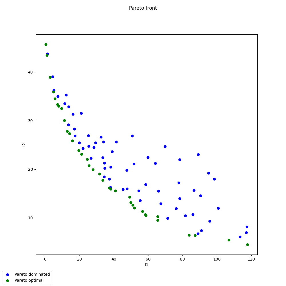
Lastly, we post-process the scenario by means of the ParetoFront
plot which generates a plot or a matrix of plots if there are more than
2 objectives, plots in blue the locally non dominated points for the current
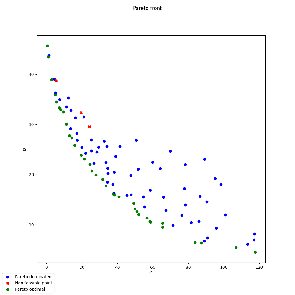
two objectives, plots in green the globally (all objectives) Pareto optimal
points. The plots in green denotes non-feasible points. Note that the user
can avoid the display of the non-feasible points.
PostFactory().execute(
    problem,
    "ParetoFront",
    save=False,
    show=False,
    show_non_feasible=False,
    objectives=["compute_binhkorn"],
    objectives_labels=["f1", "f2"],
)

PostFactory().execute(
    problem,
    "ParetoFront",
    save=False,
    show=False,
    show_non_feasible=True,
    objectives=["compute_binhkorn"],
    objectives_labels=["f1", "f2"],
)
# Workaround for HTML rendering, instead of ``show=True``
plt.show()
Total running time of the script: ( 0 minutes 0.433 seconds)