Note
Click here to download the full example code
Quadratic approximations
In this example, we illustrate the use of the QuadApprox plot
on the Sobieski’s SSBJ problem.
from __future__ import division, unicode_literals

from matplotlib import pyplot as plt
Import
The first step is to import some functions from the API and a method to get the design space.
from gemseo.api import configure_logger, create_discipline, create_scenario
from gemseo.problems.sobieski.core import SobieskiProblem

configure_logger()
Out:
<RootLogger root (INFO)>
Description
The QuadApprox post-processing
performs a quadratic approximation of a given function
from an optimization history
and plot the results as cuts of the approximation.
Create disciplines
Then, we instantiate the disciplines of the Sobieski’s SSBJ problem: Propulsion, Aerodynamics, Structure and Mission
disciplines = create_discipline(
    [
        "SobieskiPropulsion",
        "SobieskiAerodynamics",
        "SobieskiStructure",
        "SobieskiMission",
    ]
)
Create design space
We also read the design space from the SobieskiProblem.
design_space = SobieskiProblem().read_design_space()
Create and execute scenario
The next step is to build an MDO scenario in order to maximize the range, encoded ‘y_4’, with respect to the design parameters, while satisfying the inequality constraints ‘g_1’, ‘g_2’ and ‘g_3’. We can use the MDF formulation, the SLSQP optimization algorithm and a maximum number of iterations equal to 100.
scenario = create_scenario(
    disciplines,
    formulation="MDF",
    objective_name="y_4",
    maximize_objective=True,
    design_space=design_space,
)
scenario.set_differentiation_method("user")
for constraint in ["g_1", "g_2", "g_3"]:
    scenario.add_constraint(constraint, "ineq")
scenario.execute({"algo": "SLSQP", "max_iter": 10})
Out:
    INFO - 14:42:25:
    INFO - 14:42:25: *** Start MDO Scenario execution ***
    INFO - 14:42:25: MDOScenario
    INFO - 14:42:25:    Disciplines: SobieskiPropulsion SobieskiAerodynamics SobieskiStructure SobieskiMission
    INFO - 14:42:25:    MDOFormulation: MDF
    INFO - 14:42:25:    Algorithm: SLSQP
    INFO - 14:42:25: Optimization problem:
    INFO - 14:42:25:    Minimize: -y_4(x_shared, x_1, x_2, x_3)
    INFO - 14:42:25:    With respect to: x_shared, x_1, x_2, x_3
    INFO - 14:42:25:    Subject to constraints:
    INFO - 14:42:25:       g_1(x_shared, x_1, x_2, x_3) <= 0.0
    INFO - 14:42:25:       g_2(x_shared, x_1, x_2, x_3) <= 0.0
    INFO - 14:42:25:       g_3(x_shared, x_1, x_2, x_3) <= 0.0
    INFO - 14:42:25: Design space:
    INFO - 14:42:25: +----------+-------------+-------+-------------+-------+
    INFO - 14:42:25: | name     | lower_bound | value | upper_bound | type  |
    INFO - 14:42:25: +----------+-------------+-------+-------------+-------+
    INFO - 14:42:25: | x_shared |     0.01    |  0.05 |     0.09    | float |
    INFO - 14:42:25: | x_shared |    30000    | 45000 |    60000    | float |
    INFO - 14:42:25: | x_shared |     1.4     |  1.6  |     1.8     | float |
    INFO - 14:42:25: | x_shared |     2.5     |  5.5  |     8.5     | float |
    INFO - 14:42:25: | x_shared |      40     |   55  |      70     | float |
    INFO - 14:42:25: | x_shared |     500     |  1000 |     1500    | float |
    INFO - 14:42:25: | x_1      |     0.1     |  0.25 |     0.4     | float |
    INFO - 14:42:25: | x_1      |     0.75    |   1   |     1.25    | float |
    INFO - 14:42:25: | x_2      |     0.75    |   1   |     1.25    | float |
    INFO - 14:42:25: | x_3      |     0.1     |  0.5  |      1      | float |
    INFO - 14:42:25: +----------+-------------+-------+-------------+-------+
    INFO - 14:42:25: Optimization:   0%|          | 0/10 [00:00<?, ?it]
/home/docs/checkouts/readthedocs.org/user_builds/gemseo/conda/3.2.2/lib/python3.8/site-packages/scipy/sparse/linalg/dsolve/linsolve.py:407: SparseEfficiencyWarning: splu requires CSC matrix format
  warn('splu requires CSC matrix format', SparseEfficiencyWarning)
    INFO - 14:42:25: Optimization:  20%|██        | 2/10 [00:00<00:00, 52.47 it/sec, obj=2.12e+3]
    INFO - 14:42:25: Optimization:  40%|████      | 4/10 [00:00<00:00, 21.10 it/sec, obj=3.97e+3]
    INFO - 14:42:25: Optimization:  50%|█████     | 5/10 [00:00<00:00, 16.44 it/sec, obj=3.96e+3]
    INFO - 14:42:26: Optimization:  60%|██████    | 6/10 [00:00<00:00, 13.49 it/sec, obj=3.96e+3]
    INFO - 14:42:26: Optimization:  70%|███████   | 7/10 [00:00<00:00, 11.43 it/sec, obj=3.96e+3]
    INFO - 14:42:26: Optimization:  90%|█████████ | 9/10 [00:01<00:00,  9.76 it/sec, obj=3.96e+3]
    INFO - 14:42:26: Optimization: 100%|██████████| 10/10 [00:01<00:00,  9.09 it/sec, obj=3.96e+3]
    INFO - 14:42:26: Optimization result:
    INFO - 14:42:26: Objective value = 3963.595455433326
    INFO - 14:42:26: The result is feasible.
    INFO - 14:42:26: Status: None
    INFO - 14:42:26: Optimizer message: Maximum number of iterations reached. GEMSEO Stopped the driver
    INFO - 14:42:26: Number of calls to the objective function by the optimizer: 12
    INFO - 14:42:26: Constraints values:
    INFO - 14:42:26:    g_1 = [-0.01814919 -0.03340982 -0.04429875 -0.05187486 -0.05736009 -0.13720854
    INFO - 14:42:26:  -0.10279146]
    INFO - 14:42:26:    g_2 = 3.236261671801799e-05
    INFO - 14:42:26:    g_3 = [-7.67067574e-01 -2.32932426e-01 -9.19662628e-05 -1.83255000e-01]
    INFO - 14:42:26: Design space:
    INFO - 14:42:26: +----------+-------------+--------------------+-------------+-------+
    INFO - 14:42:26: | name     | lower_bound |       value        | upper_bound | type  |
    INFO - 14:42:26: +----------+-------------+--------------------+-------------+-------+
    INFO - 14:42:26: | x_shared |     0.01    | 0.0600080906541795 |     0.09    | float |
    INFO - 14:42:26: | x_shared |    30000    |       60000        |    60000    | float |
    INFO - 14:42:26: | x_shared |     1.4     |        1.4         |     1.8     | float |
    INFO - 14:42:26: | x_shared |     2.5     |        2.5         |     8.5     | float |
    INFO - 14:42:26: | x_shared |      40     |         70         |      70     | float |
    INFO - 14:42:26: | x_shared |     500     |        1500        |     1500    | float |
    INFO - 14:42:26: | x_1      |     0.1     | 0.3999993439500847 |     0.4     | float |
    INFO - 14:42:26: | x_1      |     0.75    |        0.75        |     1.25    | float |
    INFO - 14:42:26: | x_2      |     0.75    |        0.75        |     1.25    | float |
    INFO - 14:42:26: | x_3      |     0.1     | 0.156230376400943  |      1      | float |
    INFO - 14:42:26: +----------+-------------+--------------------+-------------+-------+
    INFO - 14:42:26: *** MDO Scenario run terminated in 0:00:01.110369 ***

{'algo': 'SLSQP', 'max_iter': 10}
Post-process scenario
Lastly, we post-process the scenario by means of the QuadApprox
plot which performs a quadratic approximation of a given function
from an optimization history and plot the results as cuts of the
approximation.
Tip
Each post-processing method requires different inputs and offers a variety
of customization options. Use the API function
get_post_processing_options_schema() to print a table with
the options for any post-processing algorithm.
Or refer to our dedicated page:
Options for Post-processing algorithms.
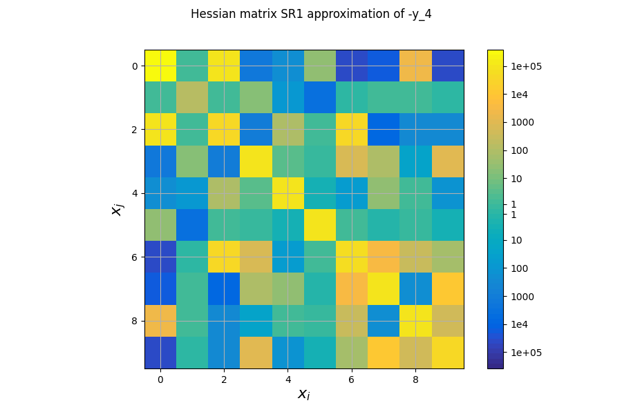
The first plot shows an approximation of the Hessian matrix \(\frac{\partial^2 f}{\partial x_i \partial x_j}\) based on the Symmetric Rank 1 method (SR1) [NW06]. The color map uses a symmetric logarithmic (symlog) scale. This plots the cross influence of the design variables on the objective function or constraints. For instance, on the last figure, the maximal second-order sensitivity is \(\frac{\partial^2 -y_4}{\partial^2 x_0} = 2.10^5\), which means that the \(x_0\) is the most influential variable. Then, the cross derivative \(\frac{\partial^2 -y_4}{\partial x_0 \partial x_2} = 5.10^4\) is positive and relatively high compared to the previous one but the combined effects of \(x_0\) and \(x_2\) are non-negligible in comparison.
scenario.post_process("QuadApprox", function="-y_4", save=False, show=False)
# Workaround for HTML rendering, instead of ``show=True``
plt.show()
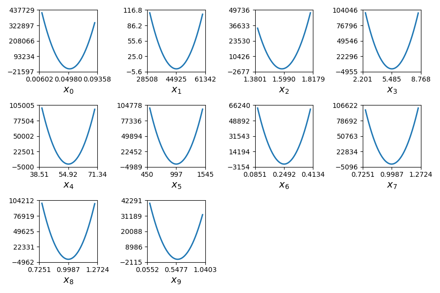
The second plot represents the quadratic approximation of the objective around the optimal solution : \(a_{i}(t)=0.5 (t-x^*_i)^2 \frac{\partial^2 f}{\partial x_i^2} + (t-x^*_i) \frac{\partial f}{\partial x_i} + f(x^*)\), where \(x^*\) is the optimal solution. This approximation highlights the sensitivity of the objective function with respect to the design variables: we notice that the design variables \(x\_1, x\_5, x\_6\) have little influence , whereas \(x\_0, x\_2, x\_9\) have a huge influence on the objective. This trend is also noted in the diagonal terms of the Hessian matrix \(\frac{\partial^2 f}{\partial x_i^2}\).
Total running time of the script: ( 0 minutes 1.840 seconds)