Tutorial: How to solve an optimization problem
Although the library |g| is dedicated to the MDO, it can also be used for mono-disciplinary optimization problems. This tutorial presents some examples on analytical test cases.
1. Optimization based on a design of experiments
Let \((P)\) be a simple optimization problem:
In this subsection, we will see how to use |g| to solve this problem \((P)\) by means of a Design Of Experiments (DOE)
1.a. Define the objective function
Firstly, by means of the create_discipline() API function,
we create a MDODiscipline of AutoPyDiscipline type
from a python function:
from gemseo.api import create_discipline

def f(x1=0., x2=0.):
    y = x1 + x2
    return y

discipline = create_discipline("AutoPyDiscipline", py_func=f)
Now, we want to minimize this MDODiscipline over a design of experiments (DOE).
1.b. Define the design space
For that, by means of the create_design_space() API function,
we define the DesignSpace \([-5, 5]\times[-5, 5]\)
by using its add_variable() method.
from gemseo.api import create_design_space

design_space = create_design_space()
design_space.add_variable("x1", 1, l_b=-5, u_b=5, var_type="integer")
design_space.add_variable("x2", 1, l_b=-5, u_b=5, var_type="integer")
1.c. Define the DOE scenario
Then, by means of the create_scenario() API function,
we define a DOEScenario from the MDODiscipline
and the DesignSpace defined above:
from gemseo.api import create_scenario

scenario = create_scenario(
    discipline, "DisciplinaryOpt", "y", design_space, scenario_type="DOE"
)
1.d. Execute the DOE scenario
Lastly, we solve the OptimizationProblem included in the DOEScenario
defined above by minimizing the objective function over a design of experiments included in the DesignSpace.
Precisely, we choose a full factorial design of size \(11^2\):
scenario.execute({"algo": "fullfact", "n_samples": 11**2})
The optimum results can be found in the execution log. It is also possible to
extract them by invoking the get_optimum() method. It
returns a dictionary containing the optimum results for the
scenario under consideration:
opt_results = scenario.get_optimum()
print("The solution of P is (x*,f(x*)) = ({}, {})".format(
    opt_results.x_opt, opt_results.f_opt
))
which yields:
The solution of P is (x*,f(x*)) = ([-5, -5], -10.0).
2. Optimization based on a quasi-Newton method by means of the library scipy
Let \((P)\) be a simple optimization problem:
In this subsection, we will see how to use |g| to solve this problem \((P)\) by means of an optimizer directly used from the library scipy.
2.a. Define the objective function
Firstly, we create the objective function and its gradient as standard python functions:
import numpy as np
from gemseo.api import create_discipline

def g(x=0):
    y = np.sin(x) - np.exp(x)
    return y

def dgdx(x=0):
    y = np.cos(x) - np.exp(x)
    return y
2.b. Minimize the objective function
Now, we can to minimize this MDODiscipline over its design space by means of
the L-BFGS-B algorithm implemented in the function scipy.optimize.fmin_l_bfgs_b.
from scipy import optimize

x_0 = -0.5 * np.ones(1)
opt = optimize.fmin_l_bfgs_b(g, x_0, fprime=dgdx, bounds=[(-.2, 2.)])
x_opt, f_opt, _ = opt
Then, we can display the solution of our optimization problem with the following code:
print("The solution of P is (x*,f(x*)) = ({}, {})".format(x_opt[0], f_opt[0]))
which gives:
The solution of P is (x*,f(x*)) = (-0.2, -1.01740008).
See also
You can found the scipy implementation of the L-BFGS-B algorithm by clicking here.
3. Optimization based on a quasi-Newton method by means of the GEMSEO optimization interface
Let \((P)\) be a simple optimization problem:
In this subsection, we will see how to use |g| to solve this problem \((P)\) by means of an optimizer from scipy called through the optimization interface of |g|.
3.a. Define the objective function
Firstly, by means of the create_discipline() API function,
we create a MDODiscipline of AutoPyDiscipline type
from a python function:
import numpy as np
from gemseo.api import create_discipline

def g(x=0):
    y = np.sin(x) - np.exp(x)
    return y

def dgdx(x=0):
    y = np.cos(x) - np.exp(x)
    return y

discipline = create_discipline("AutoPyDiscipline", py_func=g, py_jac=dgdx)
Now, we can to minimize this MDODiscipline over a design space,
by means of a quasi-Newton method from the initial point \(0.5\).
3.b. Define the design space
For that, by means of the create_design_space() API function,
we define the DesignSpace \([-2., 2.]\)
with initial value \(0.5\)
by using its add_variable() method.
from gemseo.api import create_design_space

design_space = create_design_space()
design_space.add_variable("x", 1, l_b=-2., u_b=2., value=-0.5 * np.ones(1))
3.c. Define the optimization problem
Then, by means of the create_scenario() API function,
we define a MDOScenario from the MDODiscipline
and the DesignSpace defined above:
from gemseo.api import create_scenario

scenario = create_scenario(
    discipline, "DisciplinaryOpt", "y", design_space, scenario_type="MDO"
)
3.d. Execute the optimization problem
Lastly, we solve the OptimizationProblem included in the MDOScenario
defined above by minimizing the objective function over the DesignSpace.
Precisely, we choose the L-BFGS-B algorithm
implemented in the function scipy.optimize.fmin_l_bfgs_b and
indirectly called by means of the class OptimizersFactory and of its function execute():
scenario.execute({"algo": "L-BFGS-B", "max_iter": 100})
The optimization results are displayed in the log file. They can also be obtained using the following code:
opt_results = scenario.get_optimum()
print("The solution of P is (x*,f(x*)) = ({}, {})".format(
    opt_results.x_opt, opt_results.f_opt
))
which yields:
The solution of P is (x*,f(x*)) = (-1.29, -1.24).
See also
You can found the scipy implementation of the L-BFGS-B algorithm algorithm by clicking here.
Tip
In order to get the list of available optimization algorithms, use:
from gemseo.api import get_available_opt_algorithms

algo_list = get_available_opt_algorithms()
print('Available algorithms: {}'.format(algo_list))
what gives:
Available algorithms: ['NLOPT_SLSQP', 'L-BFGS-B', 'SLSQP', 'NLOPT_COBYLA', 'NLOPT_BFGS', 'NLOPT_NEWUOA', 'TNC', 'P-L-BFGS-B', 'NLOPT_MMA', 'NLOPT_BOBYQA', 'ODD']
4. Saving and post-processing
After the resolution of the OptimizationProblem, we can export the results into a HDF file:
problem = scenario.formulation.opt_problem
problem.export_hdf("my_optim.hdf5")
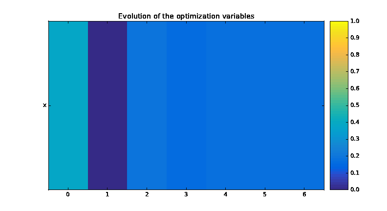
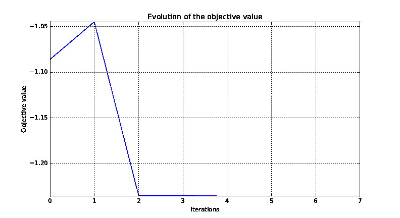
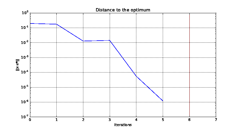
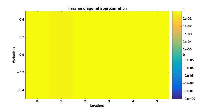
We can also post-process the optimization history by means of the function execute_post(),
either from the OptimizationProblem:
from gemseo.api import execute_post

execute_post(problem, "OptHistoryView", save=True, file_path="opt_view_with_doe")
or from the HDF file created above:
from gemseo.api import execute_post

execute_post("my_optim.hdf5", "OptHistoryView", save=True, file_path="opt_view_from_disk")
This command produces a series of PDF files: