Note
Click here to download the full example code
Constraints history
In this example, we illustrate the use of the ConstraintsHistory plot
on the Sobieski’s SSBJ problem.
from gemseo.api import configure_logger
from gemseo.api import create_discipline
from gemseo.api import create_scenario
from gemseo.problems.sobieski.core.problem import SobieskiProblem
from matplotlib import pyplot as plt
Import
The first step is to import some functions from the API and a method to get the design space.
configure_logger()
Out:
<RootLogger root (INFO)>
Description
The ConstraintsHistory post-processing
plots the constraints functions history in line charts
with violation indication by color on the background.
This plot is more precise than the constraint plot provided by the opt_history_view but scales less with the number of constraints.
Create disciplines
At this point, we instantiate the disciplines of Sobieski’s SSBJ problem: Propulsion, Aerodynamics, Structure and Mission
disciplines = create_discipline(
    [
        "SobieskiPropulsion",
        "SobieskiAerodynamics",
        "SobieskiStructure",
        "SobieskiMission",
    ]
)
Create design space
We also read the design space from the SobieskiProblem.
design_space = SobieskiProblem().design_space
Create and execute scenario
The next step is to build an MDO scenario in order to maximize the range, encoded ‘y_4’, with respect to the design parameters, while satisfying the inequality constraints ‘g_1’, ‘g_2’ and ‘g_3’. We can use the MDF formulation, the SLSQP optimization algorithm and a maximum number of iterations equal to 100.
scenario = create_scenario(
    disciplines,
    formulation="MDF",
    objective_name="y_4",
    maximize_objective=True,
    design_space=design_space,
)
scenario.set_differentiation_method("user")
all_constraints = ["g_1", "g_2", "g_3"]
for constraint in all_constraints:
    scenario.add_constraint(constraint, "ineq")
scenario.execute({"algo": "SLSQP", "max_iter": 10})
Out:
    INFO - 10:02:29:
    INFO - 10:02:29: *** Start MDOScenario execution ***
    INFO - 10:02:29: MDOScenario
    INFO - 10:02:29:    Disciplines: SobieskiPropulsion SobieskiAerodynamics SobieskiStructure SobieskiMission
    INFO - 10:02:29:    MDO formulation: MDF
    INFO - 10:02:29: Optimization problem:
    INFO - 10:02:29:    minimize -y_4(x_shared, x_1, x_2, x_3)
    INFO - 10:02:29:    with respect to x_1, x_2, x_3, x_shared
    INFO - 10:02:29:    subject to constraints:
    INFO - 10:02:29:       g_1(x_shared, x_1, x_2, x_3) <= 0.0
    INFO - 10:02:29:       g_2(x_shared, x_1, x_2, x_3) <= 0.0
    INFO - 10:02:29:       g_3(x_shared, x_1, x_2, x_3) <= 0.0
    INFO - 10:02:29:    over the design space:
    INFO - 10:02:29:    +----------+-------------+-------+-------------+-------+
    INFO - 10:02:29:    | name     | lower_bound | value | upper_bound | type  |
    INFO - 10:02:29:    +----------+-------------+-------+-------------+-------+
    INFO - 10:02:29:    | x_shared |     0.01    |  0.05 |     0.09    | float |
    INFO - 10:02:29:    | x_shared |    30000    | 45000 |    60000    | float |
    INFO - 10:02:29:    | x_shared |     1.4     |  1.6  |     1.8     | float |
    INFO - 10:02:29:    | x_shared |     2.5     |  5.5  |     8.5     | float |
    INFO - 10:02:29:    | x_shared |      40     |   55  |      70     | float |
    INFO - 10:02:29:    | x_shared |     500     |  1000 |     1500    | float |
    INFO - 10:02:29:    | x_1      |     0.1     |  0.25 |     0.4     | float |
    INFO - 10:02:29:    | x_1      |     0.75    |   1   |     1.25    | float |
    INFO - 10:02:29:    | x_2      |     0.75    |   1   |     1.25    | float |
    INFO - 10:02:29:    | x_3      |     0.1     |  0.5  |      1      | float |
    INFO - 10:02:29:    +----------+-------------+-------+-------------+-------+
    INFO - 10:02:29: Solving optimization problem with algorithm SLSQP:
    INFO - 10:02:29: ...   0%|          | 0/10 [00:00<?, ?it]
    INFO - 10:02:29: ...  20%|██        | 2/10 [00:00<00:00, 41.71 it/sec, obj=-2.12e+3]
    INFO - 10:02:30: ...  30%|███       | 3/10 [00:00<00:00, 25.08 it/sec, obj=-3.15e+3]
    INFO - 10:02:30: ...  40%|████      | 4/10 [00:00<00:00, 17.80 it/sec, obj=-3.96e+3]
    INFO - 10:02:30: ...  50%|█████     | 5/10 [00:00<00:00, 13.80 it/sec, obj=-3.98e+3]
    INFO - 10:02:30: ...  50%|█████     | 5/10 [00:00<00:00, 12.42 it/sec, obj=-3.98e+3]
    INFO - 10:02:30: Optimization result:
    INFO - 10:02:30:    Optimizer info:
    INFO - 10:02:30:       Status: 8
    INFO - 10:02:30:       Message: Positive directional derivative for linesearch
    INFO - 10:02:30:       Number of calls to the objective function by the optimizer: 6
    INFO - 10:02:30:    Solution:
    INFO - 10:02:30:       The solution is feasible.
    INFO - 10:02:30:       Objective: -3960.1367790933214
    INFO - 10:02:30:       Standardized constraints:
    INFO - 10:02:30:          g_1 = [-0.01805983 -0.03334555 -0.04424879 -0.05183405 -0.05732561 -0.13720865
    INFO - 10:02:30:  -0.10279135]
    INFO - 10:02:30:          g_2 = 2.9360600315442298e-06
    INFO - 10:02:30:          g_3 = [-0.76310174 -0.23689826 -0.00553375 -0.183255  ]
    INFO - 10:02:30:       Design space:
    INFO - 10:02:30:       +----------+-------------+---------------------+-------------+-------+
    INFO - 10:02:30:       | name     | lower_bound |        value        | upper_bound | type  |
    INFO - 10:02:30:       +----------+-------------+---------------------+-------------+-------+
    INFO - 10:02:30:       | x_shared |     0.01    | 0.06000073401500788 |     0.09    | float |
    INFO - 10:02:30:       | x_shared |    30000    |        60000        |    60000    | float |
    INFO - 10:02:30:       | x_shared |     1.4     |         1.4         |     1.8     | float |
    INFO - 10:02:30:       | x_shared |     2.5     |         2.5         |     8.5     | float |
    INFO - 10:02:30:       | x_shared |      40     |          70         |      70     | float |
    INFO - 10:02:30:       | x_shared |     500     |         1500        |     1500    | float |
    INFO - 10:02:30:       | x_1      |     0.1     |         0.4         |     0.4     | float |
    INFO - 10:02:30:       | x_1      |     0.75    |         0.75        |     1.25    | float |
    INFO - 10:02:30:       | x_2      |     0.75    |         0.75        |     1.25    | float |
    INFO - 10:02:30:       | x_3      |     0.1     |  0.1553801266337427 |      1      | float |
    INFO - 10:02:30:       +----------+-------------+---------------------+-------------+-------+
    INFO - 10:02:30: *** End MDOScenario execution (time: 0:00:00.818597) ***

{'max_iter': 10, 'algo': 'SLSQP'}
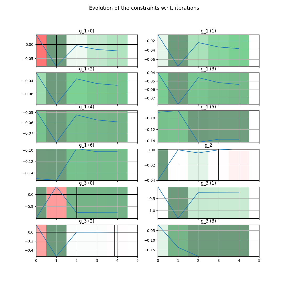
Post-process scenario
Lastly, we post-process the scenario by means of the
ConstraintsHistory plot which plots the history of constraints
passed as argument by the user. Each constraint history is represented by
a subplot where the value of the constraints is drawn by a line. Moreover,
the background color represents a qualitative view of these values: active
areas are white, violated ones are red and satisfied ones are green.
Tip
Each post-processing method requires different inputs and offers a variety
of customization options. Use the API function
get_post_processing_options_schema() to print a table with
the options for any post-processing algorithm.
Or refer to our dedicated page:
Post-processing algorithms.
scenario.post_process(
    "ConstraintsHistory", constraint_names=all_constraints, save=False, show=False
)
# Workaround for HTML rendering, instead of ``show=True``
plt.show()
Total running time of the script: ( 0 minutes 1.574 seconds)