Note
Go to the end to download the full example code
Scalable diagonal discipline
Let us consider the
SobieskiAerodynamics discipline.
We want to build its ScalableDiscipline counterpart,
using a ScalableDiagonalModel
For that, we can use a 20-length DiagonalDOE
and test different sizes of variables or different settings
for the scalable diagonal discipline.
from __future__ import annotations

from gemseo import configure_logger
from gemseo import create_discipline
from gemseo import create_scalable
from gemseo import create_scenario
from gemseo.problems.sobieski.core.problem import SobieskiProblem
Import
configure_logger()
<RootLogger root (INFO)>
Learning dataset
The first step is to build an AbstractFullCache dataset
from a DiagonalDOE.
Instantiate the discipline
For that, we instantiate the
SobieskiAerodynamics discipline
and set it up to cache all evaluations.
discipline = create_discipline("SobieskiAerodynamics")
Get the input space
We also define the input space on which to sample the discipline.
input_space = SobieskiProblem().design_space
input_names = [name for name in discipline.get_input_data_names() if name != "c_4"]
input_space.filter(input_names)
<gemseo.algos.design_space.DesignSpace object at 0x7fea48eeb5b0>
Build the DOE scenario
Lastly, we sample the discipline by means of a DOEScenario
relying on both discipline and input space.
In order to build a diagonal scalable discipline,
a DiagonalDOE must be used.
scenario = create_scenario(
    [discipline], "DisciplinaryOpt", "y_2", input_space, scenario_type="DOE"
)
for output_name in discipline.get_output_data_names():
    if output_name != "y_2":
        scenario.add_observable(output_name)
scenario.execute({"algo": "DiagonalDOE", "n_samples": 20})
    INFO - 16:25:38:
    INFO - 16:25:38: *** Start DOEScenario execution ***
    INFO - 16:25:38: DOEScenario
    INFO - 16:25:38:    Disciplines: SobieskiAerodynamics
    INFO - 16:25:38:    MDO formulation: DisciplinaryOpt
    INFO - 16:25:38: Optimization problem:
    INFO - 16:25:38:    minimize y_2(x_shared, x_2, y_32, y_12)
    INFO - 16:25:38:    with respect to x_2, x_shared, y_12, y_32
    INFO - 16:25:38:    over the design space:
    INFO - 16:25:38:    +-------------+-------------+--------------------+-------------+-------+
    INFO - 16:25:38:    | name        | lower_bound |       value        | upper_bound | type  |
    INFO - 16:25:38:    +-------------+-------------+--------------------+-------------+-------+
    INFO - 16:25:38:    | x_shared[0] |     0.01    |        0.05        |     0.09    | float |
    INFO - 16:25:38:    | x_shared[1] |    30000    |       45000        |    60000    | float |
    INFO - 16:25:38:    | x_shared[2] |     1.4     |        1.6         |     1.8     | float |
    INFO - 16:25:38:    | x_shared[3] |     2.5     |        5.5         |     8.5     | float |
    INFO - 16:25:38:    | x_shared[4] |      40     |         55         |      70     | float |
    INFO - 16:25:38:    | x_shared[5] |     500     |        1000        |     1500    | float |
    INFO - 16:25:38:    | x_2         |     0.75    |         1          |     1.25    | float |
    INFO - 16:25:38:    | y_32        |    0.235    | 0.5027962499999999 |    0.795    | float |
    INFO - 16:25:38:    | y_12[0]     |    24850    |     50606.9742     |    77250    | float |
    INFO - 16:25:38:    | y_12[1]     |     0.45    |        0.95        |     1.5     | float |
    INFO - 16:25:38:    +-------------+-------------+--------------------+-------------+-------+
    INFO - 16:25:38: Solving optimization problem with algorithm DiagonalDOE:
    INFO - 16:25:38: ...   0%|          | 0/20 [00:00<?, ?it]
    INFO - 16:25:38: ...   5%|▌         | 1/20 [00:00<00:00, 132.11 it/sec, obj=[2.48500000e+04 5.75800074e+03 4.31573408e+00]]
    INFO - 16:25:38: ...  10%|█         | 2/20 [00:00<00:00, 199.61 it/sec, obj=[2.76078947e+04 6.45112022e+03 4.27955049e+00]]
    INFO - 16:25:38: ...  15%|█▌        | 3/20 [00:00<00:00, 243.98 it/sec, obj=[3.03657895e+04 7.17864545e+03 4.23001661e+00]]
    INFO - 16:25:38: ...  20%|██        | 4/20 [00:00<00:00, 274.46 it/sec, obj=[3.31236842e+04 7.92362686e+03 4.18036902e+00]]
    INFO - 16:25:38: ...  25%|██▌       | 5/20 [00:00<00:00, 297.31 it/sec, obj=[3.58815789e+04 8.66958857e+03 4.13878683e+00]]
    INFO - 16:25:38: ...  30%|███       | 6/20 [00:00<00:00, 313.42 it/sec, obj=[3.86394737e+04 9.40253365e+03 4.10947465e+00]]
    INFO - 16:25:38: ...  35%|███▌      | 7/20 [00:00<00:00, 326.96 it/sec, obj=[4.13973684e+04 1.01086635e+04 4.09523655e+00]]
    INFO - 16:25:38: ...  40%|████      | 8/20 [00:00<00:00, 337.66 it/sec, obj=[4.41552632e+04 1.07748595e+04 4.09798968e+00]]
    INFO - 16:25:38: ...  45%|████▌     | 9/20 [00:00<00:00, 346.69 it/sec, obj=[4.69131579e+04 1.13905076e+04 4.11861872e+00]]
    INFO - 16:25:38: ...  50%|█████     | 10/20 [00:00<00:00, 354.35 it/sec, obj=[4.96710526e+04 1.19440252e+04 4.15865270e+00]]
    INFO - 16:25:38: ...  55%|█████▌    | 11/20 [00:00<00:00, 360.65 it/sec, obj=[5.24289474e+04 1.24253852e+04 4.21950279e+00]]
    INFO - 16:25:38: ...  60%|██████    | 12/20 [00:00<00:00, 363.65 it/sec, obj=[5.51868421e+04 1.28262516e+04 4.30264771e+00]]
    INFO - 16:25:38: ...  65%|██████▌   | 13/20 [00:00<00:00, 368.49 it/sec, obj=[5.79447368e+04 1.31400641e+04 4.40977580e+00]]
    INFO - 16:25:38: ...  70%|███████   | 14/20 [00:00<00:00, 372.95 it/sec, obj=[6.07026316e+04 1.33620772e+04 4.54290381e+00]]
    INFO - 16:25:38: ...  75%|███████▌  | 15/20 [00:00<00:00, 377.01 it/sec, obj=[6.34605263e+04 1.34893612e+04 4.70448714e+00]]
    INFO - 16:25:38: ...  80%|████████  | 16/20 [00:00<00:00, 380.57 it/sec, obj=[6.62184211e+04 1.35166373e+04 4.89903071e+00]]
    INFO - 16:25:38: ...  85%|████████▌ | 17/20 [00:00<00:00, 383.77 it/sec, obj=[6.89763158e+04 1.34436796e+04 5.13076164e+00]]
    INFO - 16:25:38: ...  90%|█████████ | 18/20 [00:00<00:00, 386.42 it/sec, obj=[7.17342105e+04 1.32763007e+04 5.40317758e+00]]
    INFO - 16:25:38: ...  95%|█████████▌| 19/20 [00:00<00:00, 389.22 it/sec, obj=[7.44921053e+04 1.30407235e+04 5.71226782e+00]]
    INFO - 16:25:38: ... 100%|██████████| 20/20 [00:00<00:00, 391.48 it/sec, obj=[7.72500000e+04 1.27392070e+04 6.06395673e+00]]
    INFO - 16:25:38: Optimization result:
    INFO - 16:25:38:    Optimizer info:
    INFO - 16:25:38:       Status: None
    INFO - 16:25:38:       Message: None
    INFO - 16:25:38:       Number of calls to the objective function by the optimizer: 20
    INFO - 16:25:38:    Solution:
    INFO - 16:25:38:       Objective: 25508.372961119574
    INFO - 16:25:38:       Design space:
    INFO - 16:25:38:       +-------------+-------------+-------+-------------+-------+
    INFO - 16:25:38:       | name        | lower_bound | value | upper_bound | type  |
    INFO - 16:25:38:       +-------------+-------------+-------+-------------+-------+
    INFO - 16:25:38:       | x_shared[0] |     0.01    |  0.01 |     0.09    | float |
    INFO - 16:25:38:       | x_shared[1] |    30000    | 30000 |    60000    | float |
    INFO - 16:25:38:       | x_shared[2] |     1.4     |  1.4  |     1.8     | float |
    INFO - 16:25:38:       | x_shared[3] |     2.5     |  2.5  |     8.5     | float |
    INFO - 16:25:38:       | x_shared[4] |      40     |   40  |      70     | float |
    INFO - 16:25:38:       | x_shared[5] |     500     |  500  |     1500    | float |
    INFO - 16:25:38:       | x_2         |     0.75    |  0.75 |     1.25    | float |
    INFO - 16:25:38:       | y_32        |    0.235    | 0.235 |    0.795    | float |
    INFO - 16:25:38:       | y_12[0]     |    24850    | 24850 |    77250    | float |
    INFO - 16:25:38:       | y_12[1]     |     0.45    |  0.45 |     1.5     | float |
    INFO - 16:25:38:       +-------------+-------------+-------+-------------+-------+
    INFO - 16:25:38: *** End DOEScenario execution (time: 0:00:00.069167) ***

{'eval_jac': False, 'n_samples': 20, 'algo': 'DiagonalDOE'}
Scalable diagonal discipline
Build the scalable discipline
The second step is to build a ScalableDiscipline,
using a ScalableDiagonalModel and the database
converted to a Dataset.
dataset = scenario.to_dataset(opt_naming=False)
scalable = create_scalable("ScalableDiagonalModel", dataset)
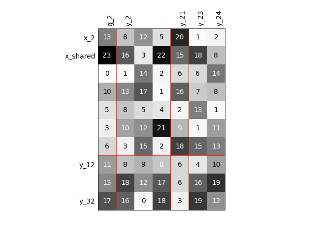
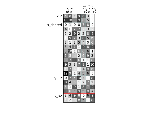
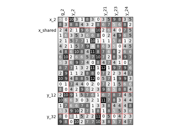
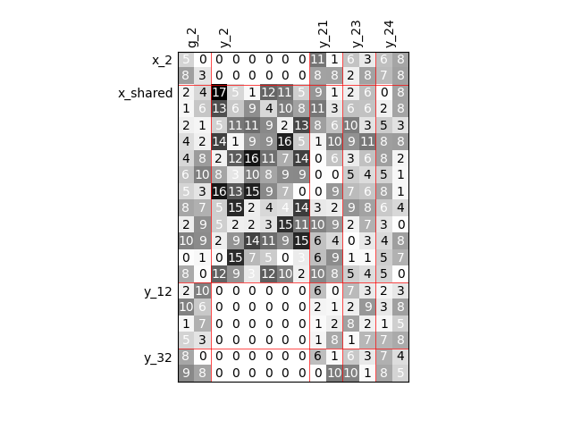
Visualize the input-output dependencies
We can easily access the underlying ScalableDiagonalModel
and plot the corresponding input-output dependency matrix
where the level of gray and the number (in [0,100]) represent
the degree of dependency between inputs and outputs.
Input are on the left while outputs are at the top.
More precisely, for a given output component located at the top of the graph,
these degrees are contributions to the output component and they add up to 1.
In other words, a degree expresses this contribution in percentage
and for a given column, the elements add up to 100.
scalable.scalable_model.plot_dependency(save=False, show=True)
'None'
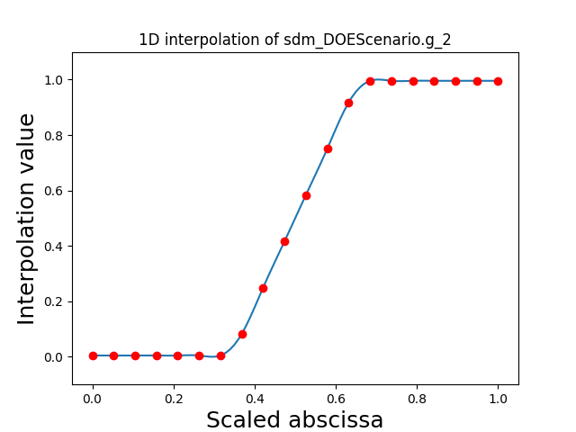
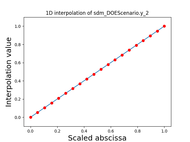
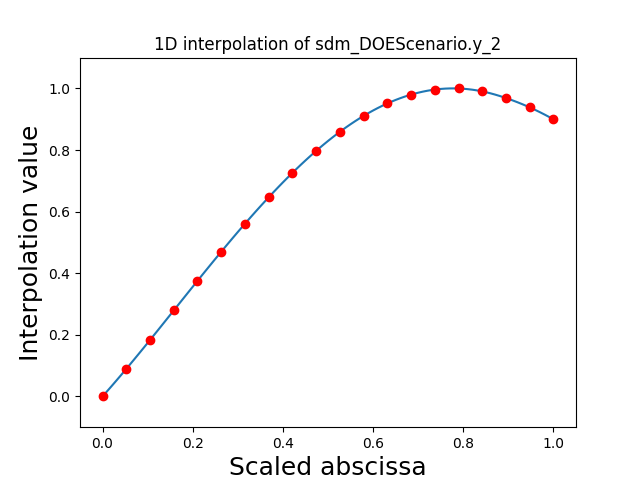
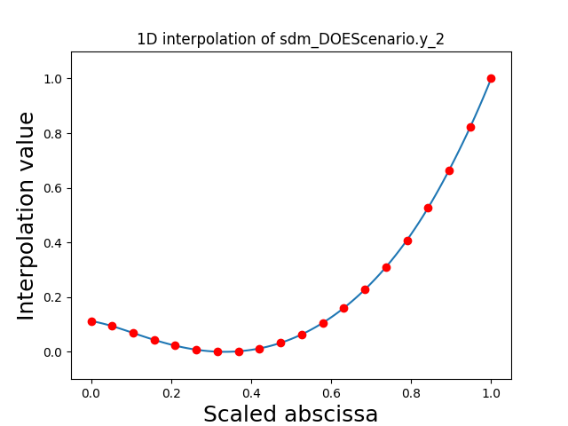
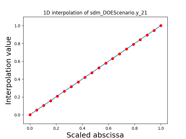
Visualize the 1D interpolations
For every output, we can also visualize a spline interpolation of the output samples over the diagonal of the input space.
scalable.scalable_model.plot_1d_interpolations(save=False, show=True)


[]
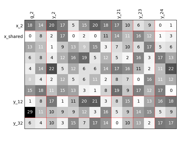
Increased problem dimension
We can repeat the construction of the scalable discipline for different sizes of variables and visualize the input-output dependency matrices.
Twice as many inputs
For example, we can increase the size of each input by a factor of 2.
sizes = {name: dataset.variable_names_to_n_components[name] * 2 for name in input_names}
scalable = create_scalable("ScalableDiagonalModel", dataset, sizes)
scalable.scalable_model.plot_dependency(save=False, show=True)
'None'
Twice as many outputs
Or we can increase the size of each output by a factor of 2.
sizes = {
    name: discipline.cache.names_to_sizes[name] * 2
    for name in discipline.get_output_data_names()
}
scalable = create_scalable("ScalableDiagonalModel", dataset, sizes)
scalable.scalable_model.plot_dependency(save=False, show=True)
'None'
Twice as many variables
Or we can increase the size of each input and each output by a factor of 2.
names = input_names + list(discipline.get_output_data_names())
sizes = {name: dataset.variable_names_to_n_components[name] * 2 for name in names}
scalable = create_scalable("ScalableDiagonalModel", dataset, sizes)
scalable.scalable_model.plot_dependency(save=False, show=True)
'None'
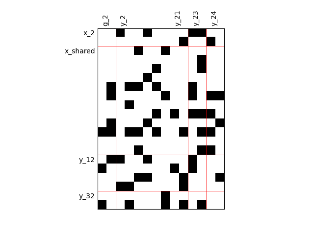
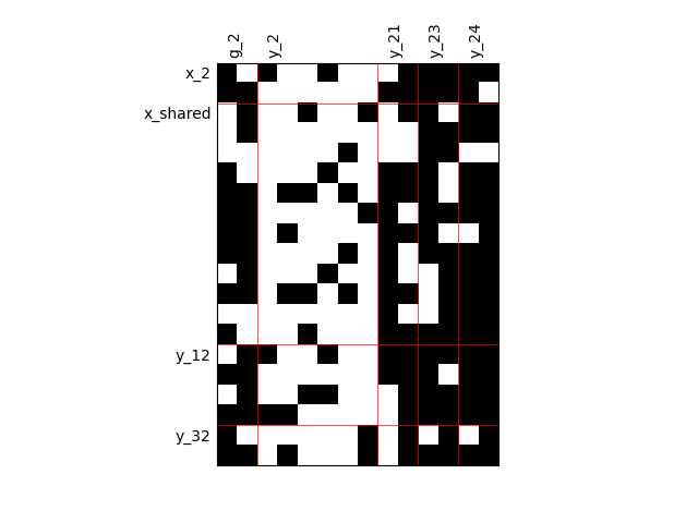
Binary IO dependencies
By default, any output component depends on any input component with a random level. We can also consider sparser input-output dependency by means of binary input-output dependency matrices. For that, we have to set the value of the fill factor which represents the part of connection between inputs and outputs. Then, a connection is represented by a black square while an absence of connection is presented by a white one. When the fill factor is equal to 1, any input is connected to any output. Conversely, when the fill factor is equal to 0, there is not a single connection between inputs and outputs.
Fill factor = 0.2
scalable = create_scalable("ScalableDiagonalModel", dataset, sizes, fill_factor=0.2)
scalable.scalable_model.plot_dependency(save=False, show=True)
'None'
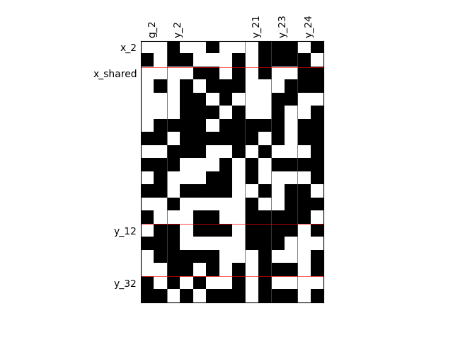
Fill factor = 0.5
scalable = create_scalable("ScalableDiagonalModel", dataset, sizes, fill_factor=0.5)
scalable.scalable_model.plot_dependency(save=False, show=True)
'None'
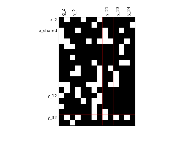
Fill factor = 0.8
scalable = create_scalable("ScalableDiagonalModel", dataset, sizes, fill_factor=0.8)
scalable.scalable_model.plot_dependency(save=False, show=True)
'None'
Heterogeneous dependencies
scalable = create_scalable(
    "ScalableDiagonalModel", dataset, sizes, fill_factor={"y_2": 0.2}
)
scalable.scalable_model.plot_dependency(save=False, show=True)
'None'
Group dependencies
scalable = create_scalable(
    "ScalableDiagonalModel", dataset, sizes, group_dep={"y_2": ["x_shared"]}
)
scalable.scalable_model.plot_dependency(save=False, show=True)
'None'
Total running time of the script: ( 0 minutes 4.061 seconds)