Self-Organizing Map

In this example, we illustrate the use of the SOM plot on the Sobieski’s SSBJ problem.

from __future__ import annotations

from gemseo import configure_logger
from gemseo import create_discipline
from gemseo import create_scenario
from gemseo.problems.sobieski.core.problem import SobieskiProblem

Import

The first step is to import some high-level functions and a method to get the design space.

configure_logger()

<RootLogger root (INFO)>

Description

The SOM post-processing performs a Self Organizing Map clustering on the optimization history. A SOM is a 2D representation of a design of experiments which requires dimensionality reduction since it may be in a very high dimension.

A SOM is built by using an unsupervised artificial neural network [KSH01]. A map of size n_x.n_y is generated, where n_x is the number of neurons in the \(x\) direction and n_y is the number of neurons in the \(y\) direction. The design space (whatever the dimension) is reduced to a 2D representation based on n_x.n_y neurons. Samples are clustered to a neuron when their design variables are close in terms of their L2 norm. A neuron is always located at the same place on a map. Each neuron is colored according to the average value for a given criterion. This helps to qualitatively analyze whether parts of the design space are good according to some criteria and not for others, and where compromises should be made. A white neuron has no sample associated with it: not enough evaluations were provided to train the SOM.

SOM’s provide a qualitative view of the objective function, the constraints, and of their relative behaviors.

Create disciplines

At this point, we instantiate the disciplines of Sobieski’s SSBJ problem: Propulsion, Aerodynamics, Structure and Mission

disciplines = create_discipline(
    [
        "SobieskiPropulsion",
        "SobieskiAerodynamics",
        "SobieskiStructure",
        "SobieskiMission",
    ]
)

Create design space

We also read the design space from the SobieskiProblem.

design_space = SobieskiProblem().design_space

Create and execute scenario

The next step is to build an MDO scenario in order to maximize the range, encoded ‘y_4’, with respect to the design parameters, while satisfying the inequality constraints ‘g_1’, ‘g_2’ and ‘g_3’. We can use the MDF formulation, the Monte Carlo DOE algorithm and 30 samples.

scenario = create_scenario(
    disciplines,
    formulation="MDF",
    objective_name="y_4",
    maximize_objective=True,
    design_space=design_space,
    scenario_type="DOE",
)
scenario.set_differentiation_method()
for constraint in ["g_1", "g_2", "g_3"]:
    scenario.add_constraint(constraint, "ineq")
scenario.execute({"algo": "OT_MONTE_CARLO", "n_samples": 30})

    INFO - 08:41:23:
    INFO - 08:41:23: *** Start DOEScenario execution ***
    INFO - 08:41:23: DOEScenario
    INFO - 08:41:23:    Disciplines: SobieskiAerodynamics SobieskiMission SobieskiPropulsion SobieskiStructure
    INFO - 08:41:23:    MDO formulation: MDF
    INFO - 08:41:23: Optimization problem:
    INFO - 08:41:23:    minimize -y_4(x_shared, x_1, x_2, x_3)
    INFO - 08:41:23:    with respect to x_1, x_2, x_3, x_shared
    INFO - 08:41:23:    subject to constraints:
    INFO - 08:41:23:       g_1(x_shared, x_1, x_2, x_3) <= 0.0
    INFO - 08:41:23:       g_2(x_shared, x_1, x_2, x_3) <= 0.0
    INFO - 08:41:23:       g_3(x_shared, x_1, x_2, x_3) <= 0.0
    INFO - 08:41:23:    over the design space:
    INFO - 08:41:23:    +-------------+-------------+-------+-------------+-------+
    INFO - 08:41:23:    | name        | lower_bound | value | upper_bound | type  |
    INFO - 08:41:23:    +-------------+-------------+-------+-------------+-------+
    INFO - 08:41:23:    | x_shared[0] |     0.01    |  0.05 |     0.09    | float |
    INFO - 08:41:23:    | x_shared[1] |    30000    | 45000 |    60000    | float |
    INFO - 08:41:23:    | x_shared[2] |     1.4     |  1.6  |     1.8     | float |
    INFO - 08:41:23:    | x_shared[3] |     2.5     |  5.5  |     8.5     | float |
    INFO - 08:41:23:    | x_shared[4] |      40     |   55  |      70     | float |
    INFO - 08:41:23:    | x_shared[5] |     500     |  1000 |     1500    | float |
    INFO - 08:41:23:    | x_1[0]      |     0.1     |  0.25 |     0.4     | float |
    INFO - 08:41:23:    | x_1[1]      |     0.75    |   1   |     1.25    | float |
    INFO - 08:41:23:    | x_2         |     0.75    |   1   |     1.25    | float |
    INFO - 08:41:23:    | x_3         |     0.1     |  0.5  |      1      | float |
    INFO - 08:41:23:    +-------------+-------------+-------+-------------+-------+
    INFO - 08:41:23: Solving optimization problem with algorithm OT_MONTE_CARLO:
    INFO - 08:41:23: ...   0%|          | 0/30 [00:00<?, ?it]
    INFO - 08:41:23: ...   3%|▎         | 1/30 [00:00<00:02,  9.80 it/sec, obj=-166]
    INFO - 08:41:23: ...   7%|▋         | 2/30 [00:00<00:01, 14.33 it/sec, obj=-484]
    INFO - 08:41:23: ...  10%|█         | 3/30 [00:00<00:01, 16.93 it/sec, obj=-481]
    INFO - 08:41:23: ...  13%|█▎        | 4/30 [00:00<00:01, 18.65 it/sec, obj=-384]
    INFO - 08:41:23: ...  17%|█▋        | 5/30 [00:00<00:01, 19.92 it/sec, obj=-1.14e+3]
    INFO - 08:41:23: ...  20%|██        | 6/30 [00:00<00:01, 20.87 it/sec, obj=-290]
    INFO - 08:41:23: ...  23%|██▎       | 7/30 [00:00<00:01, 21.33 it/sec, obj=-630]
    INFO - 08:41:23: ...  27%|██▋       | 8/30 [00:00<00:01, 21.46 it/sec, obj=-346]
    INFO - 08:41:23: ...  30%|███       | 9/30 [00:00<00:00, 21.76 it/sec, obj=-626]
    INFO - 08:41:23: ...  33%|███▎      | 10/30 [00:00<00:00, 22.02 it/sec, obj=-621]
    INFO - 08:41:23: ...  37%|███▋      | 11/30 [00:00<00:00, 22.22 it/sec, obj=-280]
    INFO - 08:41:23: ...  40%|████      | 12/30 [00:00<00:00, 21.88 it/sec, obj=-288]
    INFO - 08:41:23: ...  43%|████▎     | 13/30 [00:00<00:00, 21.61 it/sec, obj=-257]
    INFO - 08:41:23: ...  47%|████▋     | 14/30 [00:00<00:00, 21.36 it/sec, obj=-367]
    INFO - 08:41:23: ...  50%|█████     | 15/30 [00:00<00:00, 21.30 it/sec, obj=-1.08e+3]
    INFO - 08:41:24: ...  53%|█████▎    | 16/30 [00:00<00:00, 21.46 it/sec, obj=-344]
    INFO - 08:41:24: ...  57%|█████▋    | 17/30 [00:00<00:00, 21.38 it/sec, obj=-368]
    INFO - 08:41:24: ...  60%|██████    | 18/30 [00:00<00:00, 21.32 it/sec, obj=-253]
    INFO - 08:41:24: ...  63%|██████▎   | 19/30 [00:00<00:00, 21.19 it/sec, obj=-129]
    INFO - 08:41:24: ...  67%|██████▋   | 20/30 [00:00<00:00, 21.17 it/sec, obj=-1.07e+3]
    INFO - 08:41:24: ...  70%|███████   | 21/30 [00:00<00:00, 21.39 it/sec, obj=-341]
    INFO - 08:41:24: ...  73%|███████▎  | 22/30 [00:01<00:00, 21.52 it/sec, obj=-1e+3]
    INFO - 08:41:24: ...  77%|███████▋  | 23/30 [00:01<00:00, 21.22 it/sec, obj=-586]
    INFO - 08:41:24: ...  80%|████████  | 24/30 [00:01<00:00, 21.35 it/sec, obj=-483]
    INFO - 08:41:24: ...  83%|████████▎ | 25/30 [00:01<00:00, 21.53 it/sec, obj=-392]
    INFO - 08:41:24: ...  87%|████████▋ | 26/30 [00:01<00:00, 21.71 it/sec, obj=-406]
    INFO - 08:41:24: ...  90%|█████████ | 27/30 [00:01<00:00, 21.60 it/sec, obj=-207]
    INFO - 08:41:24: ...  93%|█████████▎| 28/30 [00:01<00:00, 21.76 it/sec, obj=-702]
    INFO - 08:41:24: ...  97%|█████████▋| 29/30 [00:01<00:00, 21.99 it/sec, obj=-423]
    INFO - 08:41:24: ... 100%|██████████| 30/30 [00:01<00:00, 22.07 it/sec, obj=-664]
    INFO - 08:41:24: Optimization result:
    INFO - 08:41:24:    Optimizer info:
    INFO - 08:41:24:       Status: None
    INFO - 08:41:24:       Message: None
    INFO - 08:41:24:       Number of calls to the objective function by the optimizer: 30
    INFO - 08:41:24:    Solution:
    INFO - 08:41:24:       The solution is feasible.
    INFO - 08:41:24:       Objective: -367.45728393799953
    INFO - 08:41:24:       Standardized constraints:
    INFO - 08:41:24:          g_1 = [-0.02478574 -0.00310924 -0.00855146 -0.01702654 -0.02484732 -0.04764585
    INFO - 08:41:24:  -0.19235415]
    INFO - 08:41:24:          g_2 = -0.09000000000000008
    INFO - 08:41:24:          g_3 = [-0.98722984 -0.01277016 -0.60760341 -0.0557087 ]
    INFO - 08:41:24:       Design space:
    INFO - 08:41:24:       +-------------+-------------+---------------------+-------------+-------+
    INFO - 08:41:24:       | name        | lower_bound |        value        | upper_bound | type  |
    INFO - 08:41:24:       +-------------+-------------+---------------------+-------------+-------+
    INFO - 08:41:24:       | x_shared[0] |     0.01    | 0.01230934749207792 |     0.09    | float |
    INFO - 08:41:24:       | x_shared[1] |    30000    |  43456.87364611478  |    60000    | float |
    INFO - 08:41:24:       | x_shared[2] |     1.4     |  1.731884935123487  |     1.8     | float |
    INFO - 08:41:24:       | x_shared[3] |     2.5     |  3.894765253193514  |     8.5     | float |
    INFO - 08:41:24:       | x_shared[4] |      40     |  57.92631048228255  |      70     | float |
    INFO - 08:41:24:       | x_shared[5] |     500     |  520.4048463450415  |     1500    | float |
    INFO - 08:41:24:       | x_1[0]      |     0.1     |  0.3994784918586811 |     0.4     | float |
    INFO - 08:41:24:       | x_1[1]      |     0.75    |  0.9500312867674923 |     1.25    | float |
    INFO - 08:41:24:       | x_2         |     0.75    |  1.205851870260564  |     1.25    | float |
    INFO - 08:41:24:       | x_3         |     0.1     |  0.2108042391973412 |      1      | float |
    INFO - 08:41:24:       +-------------+-------------+---------------------+-------------+-------+
    INFO - 08:41:24: *** End DOEScenario execution (time: 0:00:01.377639) ***

{'eval_jac': False, 'n_samples': 30, 'algo': 'OT_MONTE_CARLO'}

Post-process scenario

Lastly, we post-process the scenario by means of the SOM plot which performs a self organizing map clustering on optimization history.

Tip

Each post-processing method requires different inputs and offers a variety of customization options. Use the high-level function get_post_processing_options_schema() to print a table with the options for any post-processing algorithm. Or refer to our dedicated page: Post-processing algorithms.

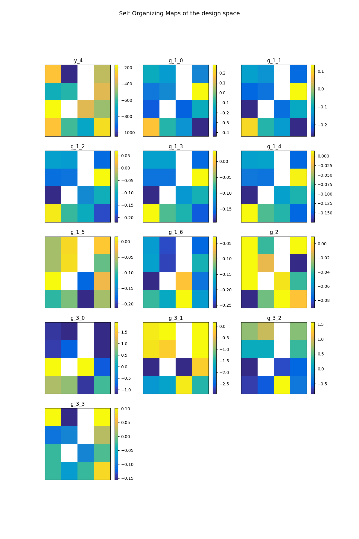
scenario.post_process("SOM", save=False, show=True)

/home/docs/checkouts/readthedocs.org/user_builds/gemseo/envs/5.0.1/lib/python3.9/site-packages/genson/schema/strategies/base.py:42: UserWarning: Schema incompatible. Keyword 'description' has conflicting values ('The width and height of the figure in inches, e.g. ``(w, h)``.\nIf ``None``, use the :attr:`.OptPostProcessor.DEFAULT_FIG_SIZE`\nof the post-processor.' vs. 'The width and height of the figure in inches, e.g. `(w, h)`.\nIf ``None``, use the :attr:`.OptPostProcessor.DEFAULT_FIG_SIZE`\nof the post-processor.'). Using 'The width and height of the figure in inches, e.g. ``(w, h)``.\nIf ``None``, use the :attr:`.OptPostProcessor.DEFAULT_FIG_SIZE`\nof the post-processor.'
  warn(('Schema incompatible. Keyword {0!r} has conflicting '
    INFO - 08:41:24: Building Self Organizing Map from optimization history:
    INFO - 08:41:24:     Number of neurons in x direction = 4
    INFO - 08:41:24:     Number of neurons in y direction = 4

<gemseo.post.som.SOM object at 0x7f8729a0e220>

Figure SOM example on the Sobieski problem. illustrates another SOM on the Sobieski use case. The optimization method is a (costly) derivative free algorithm (NLOPT_COBYLA), indeed all the relevant information for the optimization is obtained at the cost of numerous evaluations of the functions. For more details, please read the paper by [KJO+06] on wing MDO post-processing using SOM.

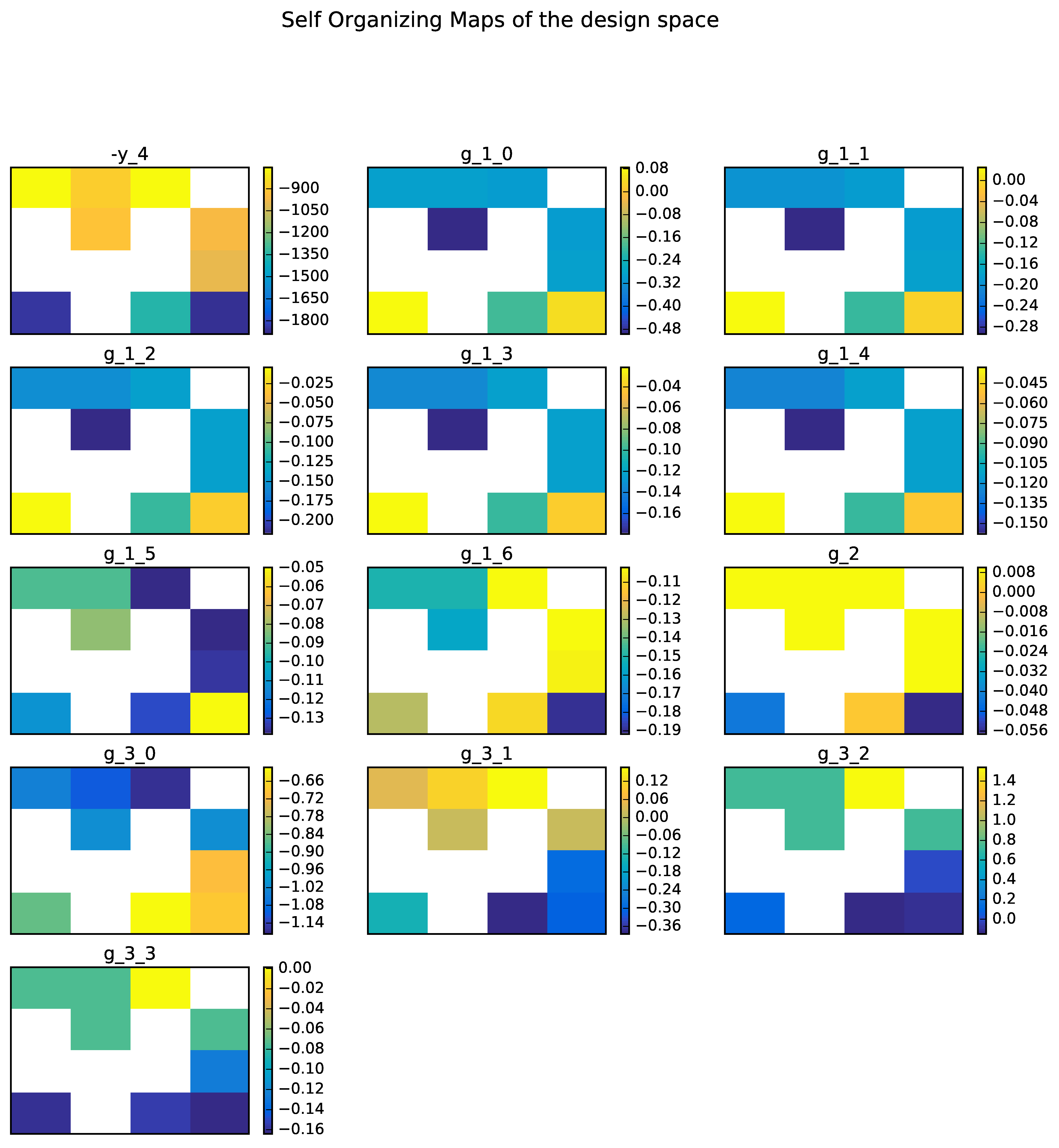
SOM example on the Sobieski problem.

A DOE may also be a good way to produce SOM maps. Figure SOM example on the Sobieski problem with a 10 000 samples DOE. shows an example with 10000 points on the same test case. This produces more relevant SOM plots.

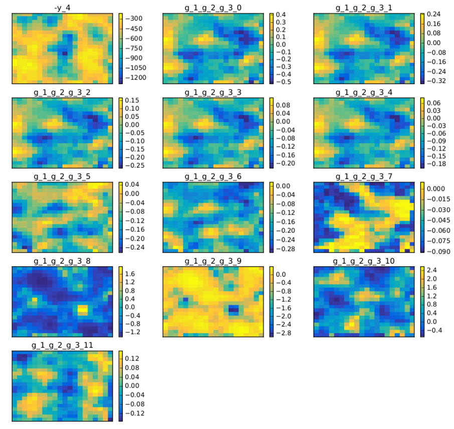
SOM example on the Sobieski problem with a 10 000 samples DOE.