Coupled derivatives and gradients computation

Introduction

The use of gradient-based methods implies the computation of the total derivatives, or Jacobian matrix, of the objective function and constraints.

\(\bf{f}=(f_0,\ldots,f_N)^T\) with respect to the design vector \(\bf{x}=(x_0,\ldots,x_n)^T\):

\[\begin{split}\frac{d\bf{f}}{d\bf{x}}=\begin{pmatrix} \displaystyle\frac{df_0}{d x_0} &\ldots&\displaystyle\frac{df_0}{dx_n}\\ \vdots&\ddots&\vdots\\ \displaystyle\frac{df_N}{d x_0} &\ldots&\displaystyle\frac{df_N}{dx_n}. \end{pmatrix}\end{split}\]

The Jacobian matrix may be either approximated (by the finite differences and complex step), or computed analytically. Both options are possible in GEMSEO.

The analytic computation of the derivatives is usually a better approach, since it is cheaper and more precise than the approximations. The tuning of the finite difference step is difficult, although some methods exist for that (set_optimal_fd_step()), and the complete MDO process has to be evaluated for each perturbed point \((\bf{x}+h_j\bf{e}_j))\), which scales badly with the number of design variables.

\[\frac{d f_i}{d x_j} = \frac{f_i(\bf{x}+h_j\bf{e}_j)-f_i(\bf{x})}{h_j}+\mathcal{O}(h_j).\]

As a result it is crucial to select an appropriate method to compute the gradient.

However, the computation of analytic derivatives is not straightforward. It requires to compute the jacobian of the objective function and constraints, that are computed by a GEMSEO process (such as a chain or a MDA), and from the derivatives provided by all the disciplines.

For weakly coupled problems, based on MDOChain, the generalized chain rule in reverse mode (from the outputs to the inputs) is used.

For the coupled problems, when the process is based on a MDA BaseMDA, a coupled adjoint approach is used, with two variants (direct or adjoint) depending on the number of design variables compared to the number of objectives and constraints.

The following section describes the coupled adjoint method.

The coupled adjoint theory

Consider the following two strongly coupled disciplines problems. The coupling variables \(\mathcal{Y_1}\) and \(\mathcal{Y_2}\), are vectors computed by each discipline, and depend on the output of the other discipline. This is formalized as two equality constraints:

\[\begin{split}\left\{ \begin{aligned} \mathcal{Y_1} = \mathcal{Y_1}(\mathbf{x}, \mathcal{Y_2})\\ \mathcal{Y_2} = \mathcal{Y_2}(\mathbf{x}, \mathcal{Y_1})\\ \end{aligned} \right.\end{split}\]

where \(\mathbf{x}\) may be a vector.

It can be rewritten in a residual form:

\[\begin{split}\left\{ \begin{aligned} \mathcal{Y_1}(\mathbf{x}, \mathcal{Y_2}) - {\mathcal{Y_1}}^\intercal = 0\\ \mathcal{Y_2}(\mathbf{x}, \mathcal{Y_1}) - {\mathcal{Y_2}}^\intercal = 0\\ \end{aligned} \right.\end{split}\]

Solving the MDA can be summarized as solving a vector residual equation:

\[\forall \mathbf{x}, \mathcal{R}(\mathbf{x}, \mathbf{\mathcal{Y}(x)}) = \mathbf{0}\]

with

\[\begin{split}\mathcal{Y} = \left\{ \begin{aligned} {\mathcal{Y_1}}^\intercal\\ {\mathcal{Y_2}}^\intercal\\ \end{aligned} \right.\end{split}\]

This assumes that the MDA is exactly solved at each iteration.

Since \(\mathcal{R}\) is a null function, its derivative with respect to \(\mathbf{x}\) is always zero, leading to:

\[\frac{\partial \mathcal{R}}{\partial \mathbf{x}} + \frac{\partial \mathcal{R}}{\partial \mathcal{Y}}~ \frac{d\mathcal{Y}}{d\mathbf{x}} = 0\]

So we can obtain the total derivative of the coupling variables :

\[\frac{d\mathcal{Y}}{d\mathbf{x}} = -\left( \frac{\partial \mathcal{R}}{\partial \mathcal{Y}} \right)^{-1} \frac{\partial \mathcal{R}}{\partial \mathbf{x}}\]

However, this linear system is very expensive when there are many design variables, so the computation of this derivative is usually not performed.

So the objective function, that depends on both the coupling and design variables \(\mathbf{f}(\mathbf{x}, \mathcal{Y}(\mathbf{x}))\), is derived:

\[\frac{d\mathbf{f}}{d\mathbf{x}} = \frac{\partial \mathbf{f}}{\partial \mathbf{x}} + \frac{\partial \mathbf{f}}{\partial \mathcal{Y}}~ \frac{d\mathcal{Y}}{d\mathbf{x}}\]

Replacing \(\frac{d\mathcal{Y}}{d\mathbf{x}}\) from the residual derivative gives:

(1)\[ \frac{d\mathbf{f}}{d\mathbf{x}} = - \frac{\partial \mathbf{f}}{\partial \mathcal{Y}}~ \left( \frac{\partial \mathcal{R}}{\partial \mathcal{Y}} \right)^{-1}~ \frac{\partial \mathcal{R}}{\partial \mathbf{x}} + \frac{\partial \mathbf{f}}{\partial \mathbf{x}}\]

Adjoint versus direct methods

The cost of evaluating the gradient of \(\mathbf{f}\) is driven by the matrix invertion \(\left( \frac{\partial \mathcal{R}}{\partial \mathcal{Y}} \right)^{-1}\). Two approaches are possible to compute the previous equation:

• The adjoint method: computation of the adjoint vector \(\bf{\lambda}\)

  \[\dfrac{d\bf{f}}{d\bf{x}} = -\underbrace{ \left[ \dfrac{\partial \bf{f}}{\partial \bf{\mathcal{Y}}} \cdot \left(\dfrac{\partial\bf{\mathcal{R}}}{\partial \bf{\mathcal{Y}}}\right)^{-1} \right]}_{\bf{\lambda}^T} \cdot \dfrac{\partial \bf{\mathcal{R}}}{\partial \bf{x}} + \dfrac{\partial \bf{f}}{\partial \bf{x}} = -\bf{\lambda}^T\cdot \dfrac{\partial \bf{\mathcal{R}}}{\partial \bf{x}} + \dfrac{\partial \bf{f}}{\partial \bf{x}}\]

  The adjoint vector is obtained by solving one linear system per output function (objective and constraint).

\[\dfrac{\partial\bf{\mathcal{R}}}{\partial \bf{\mathcal{Y}}} ^T \lambda - \dfrac{\partial \bf{f}}{\partial \bf{\mathcal{Y}}}^T = 0\]

These linear systems are the expensive part of the computation, which does not depend on the number of design variables because the equation is independent of x. The Jacobian of the functions are then obtained by a simple matrix vector product, which cost depends on the design variables number but is usually negligible.

• the direct method: linear solve of \(\dfrac{d\bf{\mathcal{Y}}}{d\bf{x}}\)

  \[\dfrac{d\bf{f}}{d\bf{x}} = -\dfrac{\partial \bf{f}}{\partial \bf{\mathcal{Y}}} \cdot \underbrace{\left[ \left(\dfrac{\partial\bf{\mathcal{R}}}{\partial \bf{\mathcal{Y}}}\right)^{-1}\cdot \dfrac{\partial \bf{\mathcal{R}}}{\partial \bf{x}}\right]}_{-d\bf{\mathcal{Y}}/d\bf{x}} + \dfrac{\partial \bf{f}}{\partial \bf{x}}\]

The computational cost is driven by the linear systems, one per design variable. It does not depend on the number of output function, so is well adapted when there are more function outputs than design variables.

The choice of which method (direct or adjoint) should be used depends on how the number \(n\) of outputs compares to the size of vector \(N\): if \(N \ll n\), the adjoint method should be used, whereas the direct method should be preferred if \(n\ll N\).

Both the direct and adjoint methods are implemented since GEMSEO v1.0.0, and the switch between the direct or adjoint method is automatic, but can be forced by the user.

Object oriented design

In GEMSEO, the JacobianAssembly class computes the derivatives of the MDAs. All MDA classes delegate the coupled derivatives computations to a JacobianAssembly instance. The MDOCouplingStructure class is responsible for the analysis of the dependencies between the MDODiscipline’s inputs and outputs, using a graph.

Many MDA algorithms are implemented in GEMSEO (Gauss-Seidel, Jacobi, Newton variants).

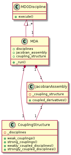
Illustration on the Sobieski SSBJ test-case

In GEMSEO, the jacobian matrix of a discipline is a dictionary of dictionaries. When wrapping the execution, a MDODiscipline._compute_jacobian() method must be defined (it overloads the generical one defined in MDODiscipline class): the jacobian matrix must be defined as MDODiscipline.jac.

def _compute_jacobian(self, inputs=None, outputs=None, mode='auto'):
    """
    Compute the partial derivatives of all outputs wrt all inputs
    """
    # Initialize all matrices to zeros
    data_names = ["y_14", "y_24", "y_34", "x_shared"]
    y_14, y_24, y_34, x_shared = self.get_inputs_by_name(data_names)
    self.jac = self.sobieski_problem.derive_blackbox_mission(x_shared,
                                                             y_14, y_24,
                                                             y_34)

The differentiation method is set by the method set_differentiation_method() of Scenario:

• for "finite_differences" (default value):

scenario.set_differentiation_method("finite_differences")

• for the "complex_step" method (each discipline must handle complex numbers):

scenario.set_differentiation_method("complex_step")

• for linearized version of the disciplines ("user"): switching from direct mode to reverse mode is automatic, depending on the number of inputs and outputs. It can also be set by the user, setting linearization_mode at "direct" or "adjoint").

scenario.set_differentiation_method("user")
for discipline in scenario.disciplines:
   discipline.linearization_mode='auto' # default, can also be 'direct' or 'adjoint'

When deriving a source code, it is very easy to make some errors or to forget to derive some terms: that is why implementation of derivation can be validated against finite differences or complex step method, by means of the method check_jacobian():

from gemseo.problems.mdo.sobieski.disciplines import SobieskiMission
from gemseo.problems.mdo.sobieski.core import SobieskiProblem

problem = SobieskiProblem("complex128")
sr = SobieskiMission("complex128")
sr.check_jacobian(indata, threshold=1e-12)

In order to be relevant, threshold value should be kept at a low level (typically \(<10^{-6}\)).