Optimal LHS vs LHS

from __future__ import annotations

import matplotlib.pyplot as plt
from gemseo.algos.doe.doe_factory import DOEFactory

n_samples = 30
n_parameters = 2

factory = DOEFactory()

lhs = factory.create("OT_LHS")
samples = lhs(n_samples, n_parameters)
samples2 = lhs(n_samples, n_parameters)

olhs = factory.create("OT_OPT_LHS")
o_samples = olhs(n_samples, n_parameters)

olhs = factory.create("OT_OPT_LHS")
o_a_samples = olhs(n_samples, n_parameters, annealing=False)

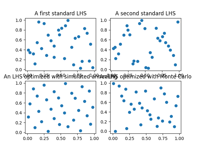
_, ax = plt.subplots(2, 2)
ax[0, 0].plot(samples[:, 0], samples[:, 1], "o")
ax[0, 0].set_title("A first standard LHS")
ax[0, 1].plot(samples2[:, 0], samples[:, 1], "o")
ax[0, 1].set_title("A second standard LHS")
ax[1, 0].plot(o_samples[:, 0], o_samples[:, 1], "o")
ax[1, 0].set_title("An LHS optimized with simulated annealing")
ax[1, 1].plot(o_a_samples[:, 0], o_a_samples[:, 1], "o")
ax[1, 1].set_title("An LHS optimized with Monte Carlo")
plt.show()