Self-Organizing Map

In this example, we illustrate the use of the SOM plot on the Sobieski’s SSBJ problem.

from __future__ import division, unicode_literals

from matplotlib import pyplot as plt

Import

The first step is to import some functions from the API and a method to get the design space.

from gemseo.api import configure_logger, create_discipline, create_scenario
from gemseo.problems.sobieski.core import SobieskiProblem

configure_logger()

Out:

<RootLogger root (INFO)>

Description

The SOM post-processing performs a Self Organizing Map clustering on the optimization history. A SOM is a 2D representation of a design of experiments which requires dimensionality reduction since it may be in a very high dimension.

A SOM is built by using an unsupervised artificial neural network [KSH01]. A map of size n_x.n_y is generated, where n_x is the number of neurons in the \(x\) direction and n_y is the number of neurons in the \(y\) direction. The design space (whatever the dimension) is reduced to a 2D representation based on n_x.n_y neurons. Samples are clustered to a neuron when their design variables are close in terms of their L2 norm. A neuron is always located at the same place on a map. Each neuron is colored according to the average value for a given criterion. This helps to qualitatively analyze whether parts of the design space are good according to some criteria and not for others, and where compromises should be made. A white neuron has no sample associated with it: not enough evaluations were provided to train the SOM.

SOM’s provide a qualitative view of the objective function, the constraints, and of their relative behaviors.

Create disciplines

At this point, we instantiate the disciplines of Sobieski’s SSBJ problem: Propulsion, Aerodynamics, Structure and Mission

disciplines = create_discipline(
    [
        "SobieskiPropulsion",
        "SobieskiAerodynamics",
        "SobieskiStructure",
        "SobieskiMission",
    ]
)

Create design space

We also read the design space from the SobieskiProblem.

design_space = SobieskiProblem().read_design_space()

Create and execute scenario

The next step is to build an MDO scenario in order to maximize the range, encoded ‘y_4’, with respect to the design parameters, while satisfying the inequality constraints ‘g_1’, ‘g_2’ and ‘g_3’. We can use the MDF formulation, the Monte Carlo DOE algorithm and 30 samples.

scenario = create_scenario(
    disciplines,
    formulation="MDF",
    objective_name="y_4",
    maximize_objective=True,
    design_space=design_space,
    scenario_type="DOE",
)
scenario.set_differentiation_method("user")
for constraint in ["g_1", "g_2", "g_3"]:
    scenario.add_constraint(constraint, "ineq")
scenario.execute({"algo": "OT_MONTE_CARLO", "n_samples": 30})

Out:

    INFO - 21:51:46:
    INFO - 21:51:46: *** Start DOE Scenario execution ***
    INFO - 21:51:46: DOEScenario
    INFO - 21:51:46:    Disciplines: SobieskiPropulsion SobieskiAerodynamics SobieskiStructure SobieskiMission
    INFO - 21:51:46:    MDOFormulation: MDF
    INFO - 21:51:46:    Algorithm: OT_MONTE_CARLO
    INFO - 21:51:46: Optimization problem:
    INFO - 21:51:46:    Minimize: -y_4(x_shared, x_1, x_2, x_3)
    INFO - 21:51:46:    With respect to: x_shared, x_1, x_2, x_3
    INFO - 21:51:46:    Subject to constraints:
    INFO - 21:51:46:       g_1(x_shared, x_1, x_2, x_3) <= 0.0
    INFO - 21:51:46:       g_2(x_shared, x_1, x_2, x_3) <= 0.0
    INFO - 21:51:46:       g_3(x_shared, x_1, x_2, x_3) <= 0.0
    INFO - 21:51:46: Generation of OT_MONTE_CARLO DOE with OpenTurns
    INFO - 21:51:46: DOE sampling:   0%|          | 0/30 [00:00<?, ?it]
    INFO - 21:51:46: DOE sampling:   7%|▋         | 2/30 [00:00<00:00, 280.71 it/sec]
    INFO - 21:51:46: DOE sampling:  17%|█▋        | 5/30 [00:00<00:00, 133.75 it/sec]
    INFO - 21:51:46: DOE sampling:  27%|██▋       | 8/30 [00:00<00:00, 84.54 it/sec]
    INFO - 21:51:47: DOE sampling:  37%|███▋      | 11/30 [00:00<00:00, 63.52 it/sec]
    INFO - 21:51:47: DOE sampling:  47%|████▋     | 14/30 [00:00<00:00, 48.38 it/sec]
    INFO - 21:51:47: DOE sampling:  57%|█████▋    | 17/30 [00:00<00:00, 39.52 it/sec]
    INFO - 21:51:47: DOE sampling:  67%|██████▋   | 20/30 [00:00<00:00, 33.87 it/sec]
    INFO - 21:51:47: DOE sampling:  77%|███████▋  | 23/30 [00:01<00:00, 29.79 it/sec]
    INFO - 21:51:47: DOE sampling:  87%|████████▋ | 26/30 [00:01<00:00, 26.06 it/sec]
    INFO - 21:51:47: DOE sampling:  97%|█████████▋| 29/30 [00:01<00:00, 23.25 it/sec]
 WARNING - 21:51:47: Optimization found no feasible point !  The least infeasible point is selected.
    INFO - 21:51:47: DOE sampling: 100%|██████████| 30/30 [00:01<00:00, 22.45 it/sec]
    INFO - 21:51:47: Optimization result:
    INFO - 21:51:47: Objective value = 617.0803511313786
    INFO - 21:51:47: The result is not feasible.
    INFO - 21:51:47: Status: None
    INFO - 21:51:47: Optimizer message: None
    INFO - 21:51:47: Number of calls to the objective function by the optimizer: 30
    INFO - 21:51:47: Constraints values:
    INFO - 21:51:47:    g_1 = [-0.48945084 -0.2922749  -0.21769656 -0.18063263 -0.15912463 -0.07434699
    INFO - 21:51:47:  -0.16565301]
    INFO - 21:51:47:    g_2 = 0.010000000000000009
    INFO - 21:51:47:    g_3 = [-0.78174978 -0.21825022 -0.11408603 -0.01907799]
    INFO - 21:51:47: Design space:
    INFO - 21:51:47: +----------+-------------+---------------------+-------------+-------+
    INFO - 21:51:47: | name     | lower_bound |        value        | upper_bound | type  |
    INFO - 21:51:47: +----------+-------------+---------------------+-------------+-------+
    INFO - 21:51:47: | x_shared |     0.01    | 0.06294679971968815 |     0.09    | float |
    INFO - 21:51:47: | x_shared |    30000    |  42733.67550603654  |    60000    | float |
    INFO - 21:51:47: | x_shared |     1.4     |  1.663874765307306  |     1.8     | float |
    INFO - 21:51:47: | x_shared |     2.5     |  5.819410624921828  |     8.5     | float |
    INFO - 21:51:47: | x_shared |      40     |  69.42919736071644  |      70     | float |
    INFO - 21:51:47: | x_shared |     500     |  1221.859441367615  |     1500    | float |
    INFO - 21:51:47: | x_1      |     0.1     |  0.1065122508792764 |     0.4     | float |
    INFO - 21:51:47: | x_1      |     0.75    |   1.09882806437771  |     1.25    | float |
    INFO - 21:51:47: | x_2      |     0.75    |   1.07969581180922  |     1.25    | float |
    INFO - 21:51:47: | x_3      |     0.1     |  0.4585171784931197 |      1      | float |
    INFO - 21:51:47: +----------+-------------+---------------------+-------------+-------+
    INFO - 21:51:47: *** DOE Scenario run terminated ***

{'eval_jac': False, 'algo': 'OT_MONTE_CARLO', 'n_samples': 30}

Post-process scenario

Lastly, we post-process the scenario by means of the SOM plot which performs a self organizing map clustering on optimization history.

Tip

Each post-processing method requires different inputs and offers a variety of customization options. Use the API function get_post_processing_options_schema() to print a table with the options for any post-processing algorithm. Or refer to our dedicated page: Options for Post-processing algorithms.

scenario.post_process("SOM", save=False, show=False)
# Workaround for HTML rendering, instead of ``show=True``
plt.show()

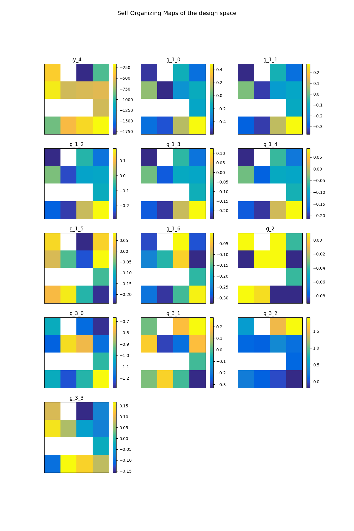
Out:

INFO - 21:51:47: Building Self Organizing Map from optimization history:
INFO - 21:51:47:     Number of neurons in x direction = 4
INFO - 21:51:47:     Number of neurons in y direction = 4

Figure SOM example on the Sobieski problem. illustrates another SOM on the Sobieski use case. The optimization method is a (costly) derivative free algorithm (NLOPT_COBYLA), indeed all the relevant information for the optimization is obtained at the cost of numerous evaluations of the functions. For more details, please read the paper by [KJO+06] on wing MDO post-processing using SOM.

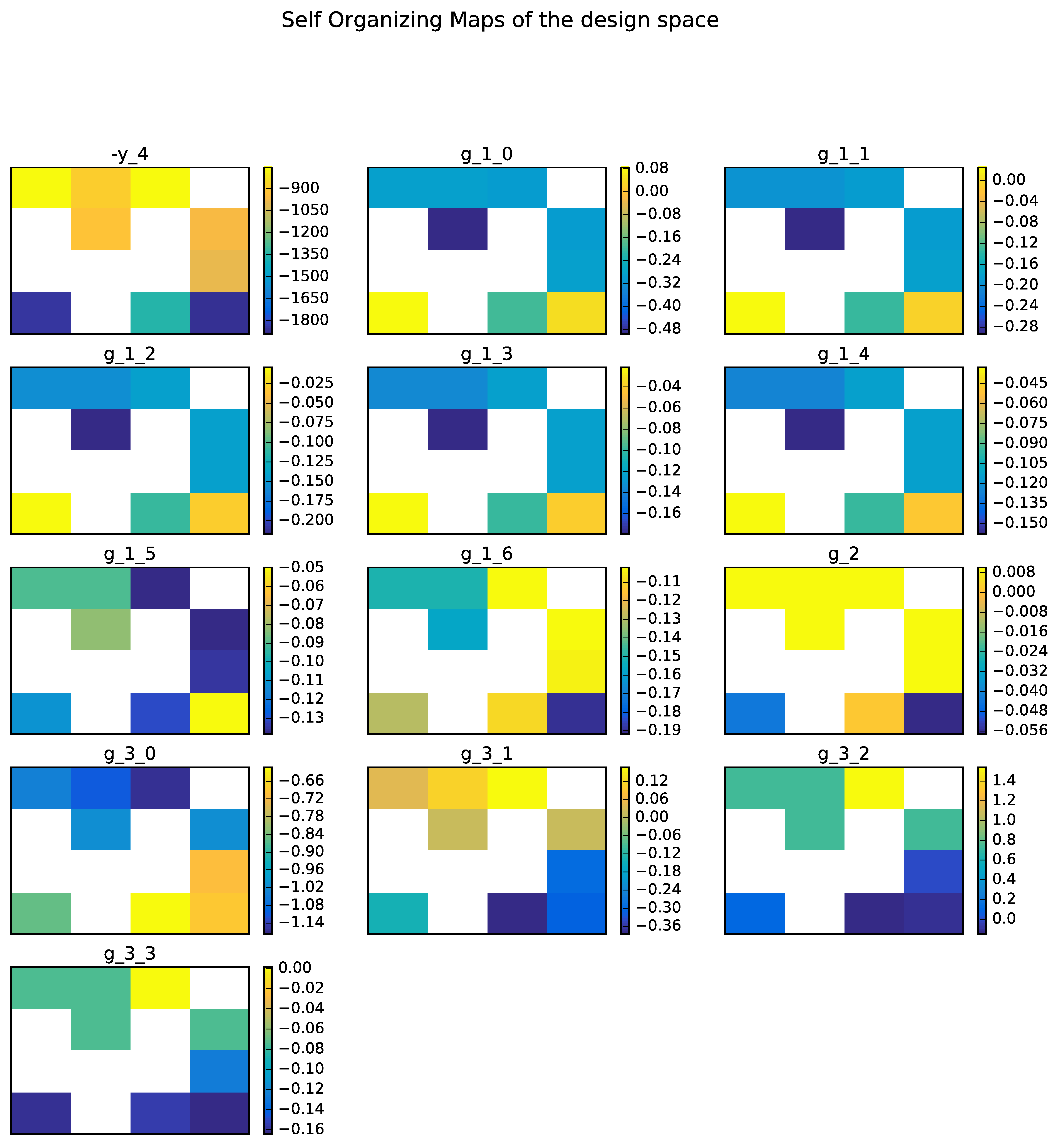
SOM example on the Sobieski problem.

A DOE may also be a good way to produce SOM maps. Figure SOM example on the Sobieski problem with a 10 000 samples DOE. shows an example with 10000 points on the same test case. This produces more relevant SOM plots.

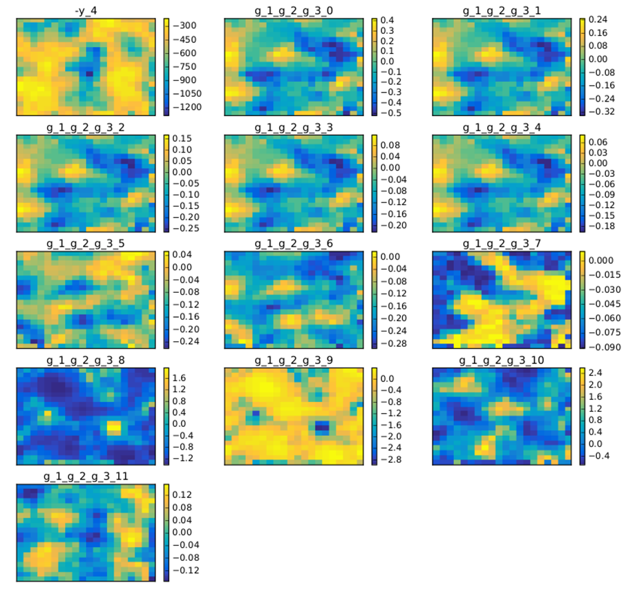
SOM example on the Sobieski problem with a 10 000 samples DOE.