Note
Click here to download the full example code
Application: Sobieski’s Super-Sonic Business Jet (MDO)
This section describes how to setup and solve the MDO problem relative to the Sobieski test case with GEMSEO.
See also
To begin with a more simple MDO problem, and have a detailed description of how to plug a test case to GEMSEO, see Tutorial: How to solve an MDO problem.
Solving with an MDF formulation
In this example, we solve the range optimization using the following MDF formulation:
The MDF formulation couples all the disciplines during the Multi Disciplinary Analyses at each optimization iteration.
All the design variables are equally treated, concatenated in a single vector and given to a single optimization algorithm as the unknowns of the problem.
There is no specific constraint due to the MDF formulation.
Only the design constraints \(g\_1\), \(g\_2\) and \(g\_3\) are added to the problem.
The objective function is the range (the \(y\_4\) variable in the model), computed after the Multi Disciplinary Analyses.
Imports
All the imports needed for the tutorials are performed here. Note that some of the imports are related to the Python 2/3 compatibility.
from gemseo.api import configure_logger
from gemseo.api import create_discipline
from gemseo.api import create_scenario
from gemseo.api import get_available_formulations
from gemseo.core.jacobian_assembly import JacobianAssembly
from gemseo.disciplines.utils import get_all_inputs
from gemseo.disciplines.utils import get_all_outputs
from gemseo.problems.sobieski.core.problem import SobieskiProblem
from matplotlib import pyplot as plt

configure_logger()
Out:
<RootLogger root (INFO)>
Step 1: Creation of MDODiscipline
To build the scenario, we first instantiate the disciplines. Here, the disciplines themselves have already been developed and interfaced with GEMSEO (see Benchmark problems).
disciplines = create_discipline(
    [
        "SobieskiPropulsion",
        "SobieskiAerodynamics",
        "SobieskiMission",
        "SobieskiStructure",
    ]
)
Tip
For the disciplines that are not interfaced with GEMSEO, the GEMSEO’s
api eases the creation of disciplines without having
to import them.
Step 2: Creation of Scenario
The scenario delegates the creation of the optimization problem to the MDO formulation.
Therefore, it needs the list of disciplines, the names of the formulation,
the name of the objective function and the design space.
The
design_space(shown below for reference, asdesign_space.txt) defines the unknowns of the optimization problem, and their bounds. It contains all the design variables needed by the MDF formulation. It can be imported from a text file, or created from scratch with the methodscreate_design_space()andadd_variable(). In this case, we will create it directly from the API.
design_space = SobieskiProblem().design_space
vi design_space.txt

name      lower_bound      value      upper_bound  type
x_shared      0.01          0.05          0.09     float
x_shared    30000.0       45000.0       60000.0    float
x_shared      1.4           1.6           1.8      float
x_shared      2.5           5.5           8.5      float
x_shared      40.0          55.0          70.0     float
x_shared     500.0         1000.0        1500.0    float
x_1           0.1           0.25          0.4      float
x_1           0.75          1.0           1.25     float
x_2           0.75          1.0           1.25     float
x_3           0.1           0.5           1.0      float
y_14        24850.0    50606.9741711    77100.0    float
y_14        -7700.0    7306.20262124    45000.0    float
y_32         0.235       0.50279625      0.795     float
y_31         2960.0    6354.32430691    10185.0    float
y_24          0.44       4.15006276      11.13     float
y_34          0.44       1.10754577       1.98     float
y_23         3365.0    12194.2671934    26400.0    float
y_21        24850.0    50606.9741711    77250.0    float
y_12        24850.0      50606.9742     77250.0    float
y_12          0.45          0.95          1.5      float
The available MDO formulations are located in the gemseo.formulations package, see Extend GEMSEO features for extending GEMSEO with other formulations.
The
formulationclassname (here,"MDF") shall be passed to the scenario to select them.The list of available formulations can be obtained by using
get_available_formulations().
get_available_formulations()
Out:
['BiLevel', 'DisciplinaryOpt', 'IDF', 'MDF']
\(y\_4\) corresponds to the
objective_name. This name must be one of the disciplines outputs, here the “SobieskiMission” discipline. The list of all outputs of the disciplines can be obtained by usingget_all_outputs():
get_all_outputs(disciplines)
get_all_inputs(disciplines)
Out:
['y_12', 'y_24', 'x_shared', 'y_14', 'y_34', 'y_31', 'c_2', 'c_3', 'x_3', 'x_2', 'y_32', 'c_1', 'y_21', 'c_4', 'c_0', 'x_1', 'y_23']
From these MDODiscipline, design space filename,
MDO formulation name and objective function name,
we build the scenario:
scenario = create_scenario(
    disciplines,
    formulation="MDF",
    maximize_objective=True,
    objective_name="y_4",
    design_space=design_space,
)
The range function (\(y\_4\)) should be maximized. However, optimizers
minimize functions by default. Which is why, when creating the scenario, the argument
maximize_objective shall be set to True.
Scenario options
We may provide additional options to the scenario:
Function derivatives. As analytical disciplinary derivatives are vailable for Sobieski test-case, they can be used instead of computing the derivatives with finite-differences or with the complex-step method. The easiest way to set a method is to let the optimizer determine it:
scenario.set_differentiation_method("user")
The default behavior of the optimizer triggers finite differences. It corresponds to:
scenario.set_differentiation_method("finite_differences",1e-7)
It it also possible to differentiate functions by means of the complex step method:
scenario.set_differentiation_method("complex_step",1e-30j)
Constraints
Similarly to the objective function, the constraints names are a subset
of the disciplines’ outputs. They can be obtained by using
get_all_outputs().
The formulation has a powerful feature to automatically dispatch the constraints
(\(g\_1, g\_2, g\_3\)) and plug them to the optimizers depending on
the formulation. To do that, we use the method
add_constraint():
for constraint in ["g_1", "g_2", "g_3"]:
    scenario.add_constraint(constraint, "ineq")
Step 3: Execution and visualization of the results
The algorithm arguments are provided as a dictionary to the execution method of the scenario:
algo_args = {"max_iter": 10, "algo": "SLSQP"}
Warning
The mandatory arguments are the maximum number of iterations and the algorithm name.
Any other options of the optimization algorithm can be prescribed through
the argument algo_options with a dictionary, e.g.
algo_args =
{"max_iter": 10, "algo": "SLSQP": "algo_options": {"ftol_rel": 1e-6}}
.
This list of available algorithm options are detailed here: Optimization algorithms.
The scenario is executed by means of the line:
scenario.execute(algo_args)
Out:
    INFO - 07:18:17:
    INFO - 07:18:17: *** Start MDOScenario execution ***
    INFO - 07:18:17: MDOScenario
    INFO - 07:18:17:    Disciplines: SobieskiPropulsion SobieskiAerodynamics SobieskiMission SobieskiStructure
    INFO - 07:18:17:    MDO formulation: MDF
    INFO - 07:18:17: Optimization problem:
    INFO - 07:18:17:    minimize -y_4(x_shared, x_1, x_2, x_3)
    INFO - 07:18:17:    with respect to x_1, x_2, x_3, x_shared
    INFO - 07:18:17:    subject to constraints:
    INFO - 07:18:17:       g_1(x_shared, x_1, x_2, x_3) <= 0.0
    INFO - 07:18:17:       g_2(x_shared, x_1, x_2, x_3) <= 0.0
    INFO - 07:18:17:       g_3(x_shared, x_1, x_2, x_3) <= 0.0
    INFO - 07:18:17:    over the design space:
    INFO - 07:18:17:    +----------+-------------+-------+-------------+-------+
    INFO - 07:18:17:    | name     | lower_bound | value | upper_bound | type  |
    INFO - 07:18:17:    +----------+-------------+-------+-------------+-------+
    INFO - 07:18:17:    | x_shared |     0.01    |  0.05 |     0.09    | float |
    INFO - 07:18:17:    | x_shared |    30000    | 45000 |    60000    | float |
    INFO - 07:18:17:    | x_shared |     1.4     |  1.6  |     1.8     | float |
    INFO - 07:18:17:    | x_shared |     2.5     |  5.5  |     8.5     | float |
    INFO - 07:18:17:    | x_shared |      40     |   55  |      70     | float |
    INFO - 07:18:17:    | x_shared |     500     |  1000 |     1500    | float |
    INFO - 07:18:17:    | x_1      |     0.1     |  0.25 |     0.4     | float |
    INFO - 07:18:17:    | x_1      |     0.75    |   1   |     1.25    | float |
    INFO - 07:18:17:    | x_2      |     0.75    |   1   |     1.25    | float |
    INFO - 07:18:17:    | x_3      |     0.1     |  0.5  |      1      | float |
    INFO - 07:18:17:    +----------+-------------+-------+-------------+-------+
    INFO - 07:18:17: Solving optimization problem with algorithm SLSQP:
    INFO - 07:18:17: ...   0%|          | 0/10 [00:00<?, ?it]
    INFO - 07:18:18: ...  20%|██        | 2/10 [00:00<00:00, 41.22 it/sec, obj=-2.12e+3]
 WARNING - 07:18:18: MDAJacobi has reached its maximum number of iterations but the normed residual 1.0259352902248124e-06 is still above the tolerance 1e-06.
    INFO - 07:18:18: ...  30%|███       | 3/10 [00:00<00:00, 23.56 it/sec, obj=-3.8e+3]
    INFO - 07:18:18: ...  40%|████      | 4/10 [00:00<00:00, 17.04 it/sec, obj=-3.96e+3]
    INFO - 07:18:18: ...  50%|█████     | 5/10 [00:00<00:00, 13.35 it/sec, obj=-3.96e+3]
    INFO - 07:18:18: ...  60%|██████    | 6/10 [00:00<00:00, 10.98 it/sec, obj=-3.96e+3]
    INFO - 07:18:19: ...  70%|███████   | 7/10 [00:01<00:00,  9.49 it/sec, obj=-4.81e+3]
    INFO - 07:18:19: ...  90%|█████████ | 9/10 [00:01<00:00,  7.90 it/sec, obj=-3.87e+3]
    INFO - 07:18:19: ... 100%|██████████| 10/10 [00:01<00:00,  7.50 it/sec, obj=-4.64e+3]
    INFO - 07:18:19: Optimization result:
    INFO - 07:18:19:    Optimizer info:
    INFO - 07:18:19:       Status: None
    INFO - 07:18:19:       Message: Maximum number of iterations reached. GEMSEO Stopped the driver
    INFO - 07:18:19:       Number of calls to the objective function by the optimizer: 12
    INFO - 07:18:19:    Solution:
    INFO - 07:18:19:       The solution is feasible.
    INFO - 07:18:19:       Objective: -3963.5118239326903
    INFO - 07:18:19:       Standardized constraints:
    INFO - 07:18:19:          g_1 = [-0.01808064 -0.03336052 -0.04426042 -0.05184355 -0.05733364 -0.13720861
    INFO - 07:18:19:  -0.10279139]
    INFO - 07:18:19:          g_2 = 9.785920617177979e-06
    INFO - 07:18:19:          g_3 = [-7.67233630e-01 -2.32766370e-01  8.55509121e-05 -1.83255000e-01]
    INFO - 07:18:19:       Design space:
    INFO - 07:18:19:       +----------+-------------+---------------------+-------------+-------+
    INFO - 07:18:19:       | name     | lower_bound |        value        | upper_bound | type  |
    INFO - 07:18:19:       +----------+-------------+---------------------+-------------+-------+
    INFO - 07:18:19:       | x_shared |     0.01    | 0.06000244648015432 |     0.09    | float |
    INFO - 07:18:19:       | x_shared |    30000    |        60000        |    60000    | float |
    INFO - 07:18:19:       | x_shared |     1.4     |         1.4         |     1.8     | float |
    INFO - 07:18:19:       | x_shared |     2.5     |         2.5         |     8.5     | float |
    INFO - 07:18:19:       | x_shared |      40     |          70         |      70     | float |
    INFO - 07:18:19:       | x_shared |     500     |         1500        |     1500    | float |
    INFO - 07:18:19:       | x_1      |     0.1     |  0.3999997783130735 |     0.4     | float |
    INFO - 07:18:19:       | x_1      |     0.75    |         0.75        |     1.25    | float |
    INFO - 07:18:19:       | x_2      |     0.75    |         0.75        |     1.25    | float |
    INFO - 07:18:19:       | x_3      |     0.1     |  0.1562581125267868 |      1      | float |
    INFO - 07:18:19:       +----------+-------------+---------------------+-------------+-------+
    INFO - 07:18:19: *** End MDOScenario execution (time: 0:00:01.346081) ***

{'max_iter': 10, 'algo': 'SLSQP'}
Post-processing options
A whole variety of visualizations may be displayed for both MDO and DOE scenarios. These features are illustrated on the SSBJ use case in How to deal with post-processing.
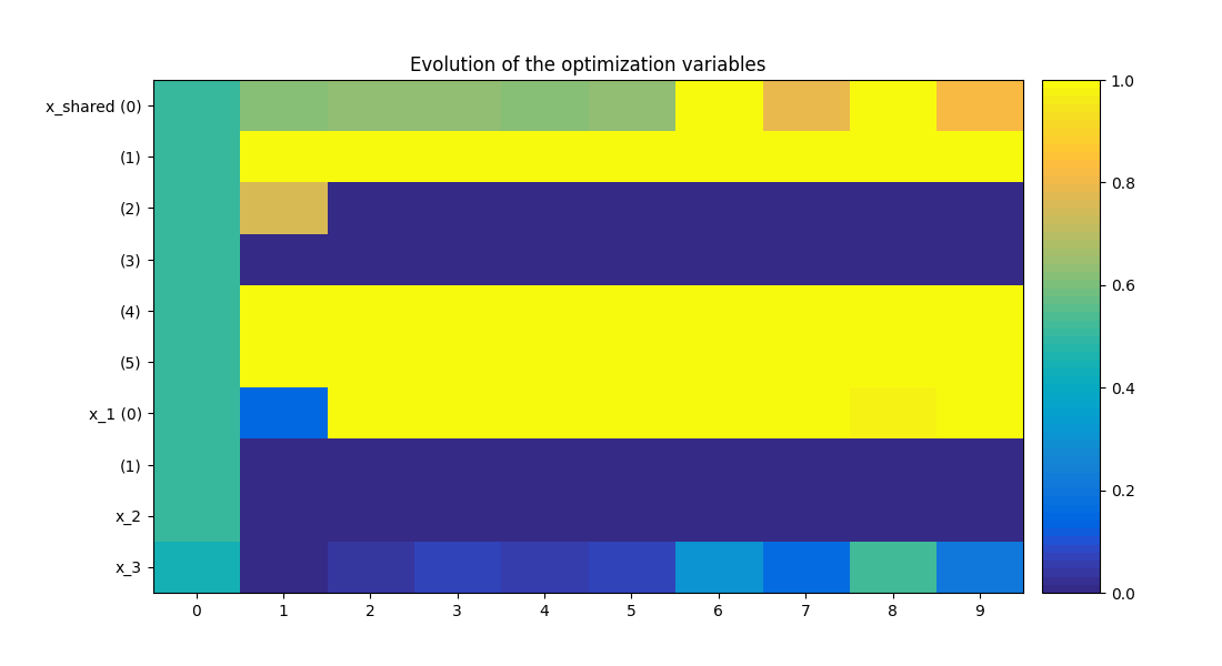
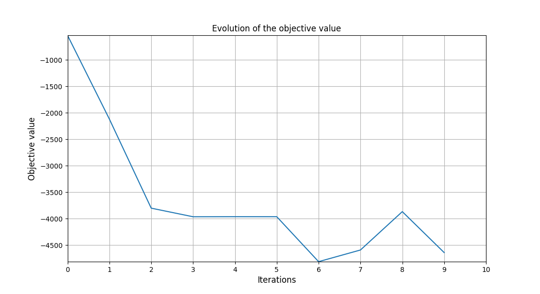
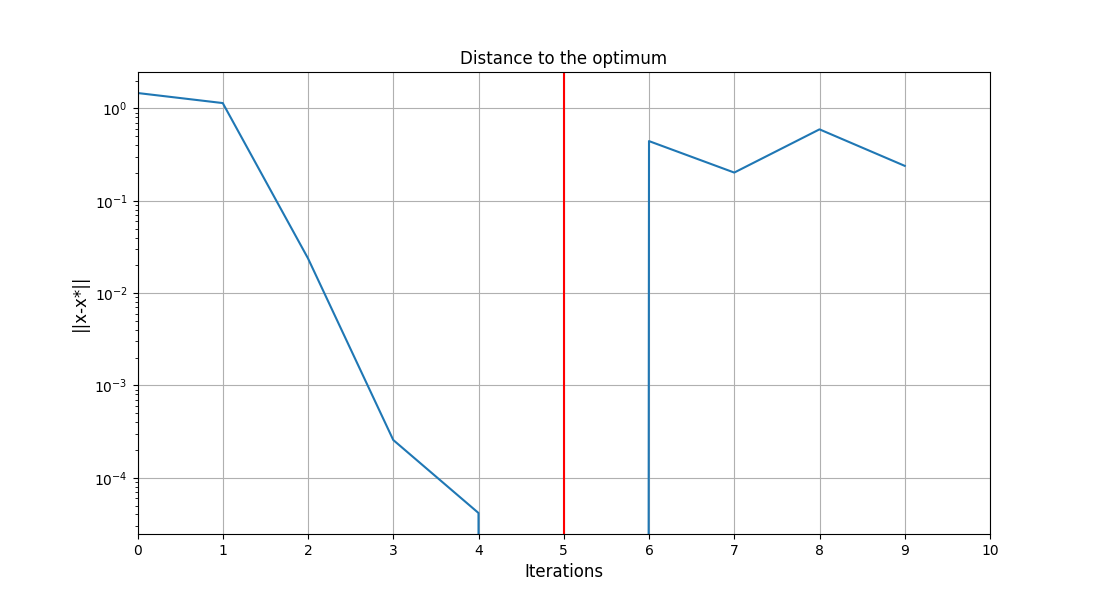
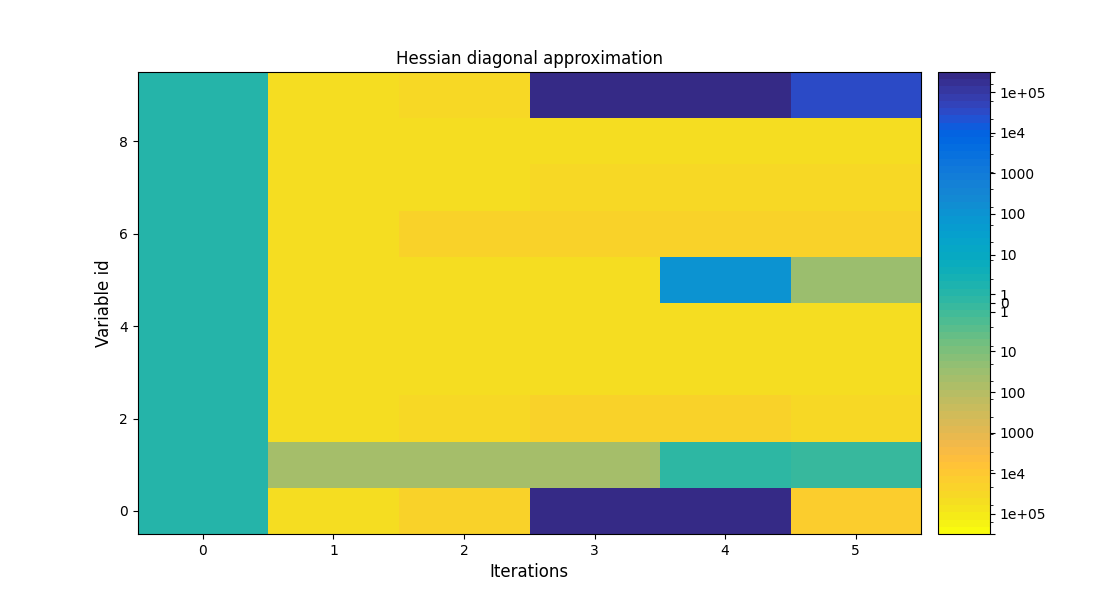
To visualize the optimization history:
scenario.post_process("OptHistoryView", save=False, show=False)
# Workaround for HTML rendering, instead of ``show=True``
plt.show()
Influence of gradient computation method on performance
As mentioned in Coupled derivatives computation, several methods are available in order to perform the gradient computations: classical finite differences, complex step and Multi Disciplinary Analyses linearization in direct or adjoint mode. These modes are automatically selected by GEMSEO to minimize the CPU time. Yet, they can be forced on demand in each Multi Disciplinary Analyses:
scenario.formulation.mda.linearization_mode = JacobianAssembly.DIRECT_MODE
scenario.formulation.mda.matrix_type = JacobianAssembly.LINEAR_OPERATOR
The method used to solve the adjoint or direct linear problem may also be selected. GEMSEO can either assemble a sparse residual Jacobian matrix of the Multi Disciplinary Analyses from the disciplines matrices. This has the advantage that LU factorizations may be stored to solve multiple right hand sides problems in a cheap way. But this requires extra memory.
scenario.formulation.mda.matrix_type = JacobianAssembly.SPARSE
scenario.formulation.mda.use_lu_fact = True
Altenatively, GEMSEO can implicitly create a matrix-vector product operator, which is sufficient for GMRES-like solvers. It avoids to create an additional data structure. This can also be mandatory if the disciplines do not provide full Jacobian matrices but only matrix-vector product operators.
scenario.formulation.mda.matrix_type = JacobianAssembly.LINEAR_OPERATOR
The next table shows the performance of each method for solving the Sobieski use case with MDF and IDF formulations. Efficiency of linearization is clearly visible has it takes from 10 to 20 times less CPU time to compute analytic derivatives of an Multi Disciplinary Analyses compared to finite difference and complex step. For IDF, improvements are less consequent, but direct linearization is more than 2.5 times faster than other methods.
Derivation Method |
Execution time (s) |
|
|---|---|---|
Finite differences |
8.22 |
1.93 |
Complex step |
18.11 |
2.07 |
Linearized (direct) |
0.90 |
0.68 |
Total running time of the script: ( 0 minutes 2.515 seconds)