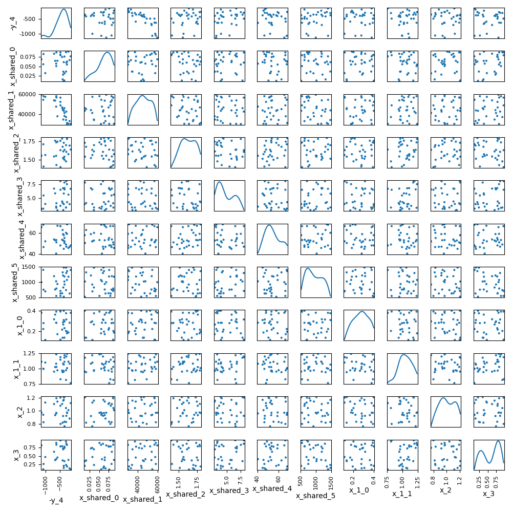
Scatter plot matrix

In this example, we illustrate the use of the ScatterPlotMatrix plot on the Sobieski’s SSBJ problem.

from gemseo.api import configure_logger
from gemseo.api import create_discipline
from gemseo.api import create_scenario
from gemseo.problems.sobieski.core.problem import SobieskiProblem
from matplotlib import pyplot as plt

Import

The first step is to import some functions from the API and a method to get the design space.

configure_logger()

Out:

<RootLogger root (INFO)>

Description

The ScatterPlotMatrix post-processing builds the scatter plot matrix among design variables and outputs functions. Each non-diagonal block represents the samples according to the x- and y- coordinates names while the diagonal ones approximate the probability distributions of the variables, using a kernel-density estimator.

Create disciplines

At this point, we instantiate the disciplines of Sobieski’s SSBJ problem: Propulsion, Aerodynamics, Structure and Mission

disciplines = create_discipline(
    [
        "SobieskiPropulsion",
        "SobieskiAerodynamics",
        "SobieskiStructure",
        "SobieskiMission",
    ]
)

Create design space

We also read the design space from the SobieskiProblem.

design_space = SobieskiProblem().design_space

Create and execute scenario

The next step is to build a DOE scenario in order to maximize the range, encoded ‘y_4’, with respect to the design parameters, while satisfying the inequality constraints ‘g_1’, ‘g_2’ and ‘g_3’. We can use the MDF formulation, the Monte Carlo DOE algorithm and 30 samples.

scenario = create_scenario(
    disciplines,
    formulation="MDF",
    objective_name="y_4",
    maximize_objective=True,
    design_space=design_space,
    scenario_type="DOE",
)
scenario.set_differentiation_method("user")
for constraint in ["g_1", "g_2", "g_3"]:
    scenario.add_constraint(constraint, "ineq")
scenario.execute({"algo": "OT_MONTE_CARLO", "n_samples": 30})

Out:

    INFO - 07:15:06:
    INFO - 07:15:06: *** Start DOEScenario execution ***
    INFO - 07:15:06: DOEScenario
    INFO - 07:15:06:    Disciplines: SobieskiPropulsion SobieskiAerodynamics SobieskiStructure SobieskiMission
    INFO - 07:15:06:    MDO formulation: MDF
    INFO - 07:15:06: Optimization problem:
    INFO - 07:15:06:    minimize -y_4(x_shared, x_1, x_2, x_3)
    INFO - 07:15:06:    with respect to x_1, x_2, x_3, x_shared
    INFO - 07:15:06:    subject to constraints:
    INFO - 07:15:06:       g_1(x_shared, x_1, x_2, x_3) <= 0.0
    INFO - 07:15:06:       g_2(x_shared, x_1, x_2, x_3) <= 0.0
    INFO - 07:15:06:       g_3(x_shared, x_1, x_2, x_3) <= 0.0
    INFO - 07:15:06:    over the design space:
    INFO - 07:15:06:    +----------+-------------+-------+-------------+-------+
    INFO - 07:15:06:    | name     | lower_bound | value | upper_bound | type  |
    INFO - 07:15:06:    +----------+-------------+-------+-------------+-------+
    INFO - 07:15:06:    | x_shared |     0.01    |  0.05 |     0.09    | float |
    INFO - 07:15:06:    | x_shared |    30000    | 45000 |    60000    | float |
    INFO - 07:15:06:    | x_shared |     1.4     |  1.6  |     1.8     | float |
    INFO - 07:15:06:    | x_shared |     2.5     |  5.5  |     8.5     | float |
    INFO - 07:15:06:    | x_shared |      40     |   55  |      70     | float |
    INFO - 07:15:06:    | x_shared |     500     |  1000 |     1500    | float |
    INFO - 07:15:06:    | x_1      |     0.1     |  0.25 |     0.4     | float |
    INFO - 07:15:06:    | x_1      |     0.75    |   1   |     1.25    | float |
    INFO - 07:15:06:    | x_2      |     0.75    |   1   |     1.25    | float |
    INFO - 07:15:06:    | x_3      |     0.1     |  0.5  |      1      | float |
    INFO - 07:15:06:    +----------+-------------+-------+-------------+-------+
    INFO - 07:15:06: Solving optimization problem with algorithm OT_MONTE_CARLO:
    INFO - 07:15:06: Generation of OT_MONTE_CARLO DOE with OpenTURNS
    INFO - 07:15:06: ...   0%|          | 0/30 [00:00<?, ?it]
    INFO - 07:15:06: ...   3%|▎         | 1/30 [00:00<00:00, 278.43 it/sec]
    INFO - 07:15:07: ...  13%|█▎        | 4/30 [00:00<00:00, 126.78 it/sec]
    INFO - 07:15:07: ...  23%|██▎       | 7/30 [00:00<00:00, 82.31 it/sec]
    INFO - 07:15:07: ...  33%|███▎      | 10/30 [00:00<00:00, 58.79 it/sec]
    INFO - 07:15:07: ...  43%|████▎     | 13/30 [00:00<00:00, 43.06 it/sec]
    INFO - 07:15:07: ...  50%|█████     | 15/30 [00:00<00:00, 36.56 it/sec]
    INFO - 07:15:07: ...  57%|█████▋    | 17/30 [00:00<00:00, 32.32 it/sec]
    INFO - 07:15:07: ...  63%|██████▎   | 19/30 [00:01<00:00, 28.64 it/sec]
    INFO - 07:15:07: ...  73%|███████▎  | 22/30 [00:01<00:00, 25.24 it/sec]
    INFO - 07:15:08: ...  80%|████████  | 24/30 [00:01<00:00, 23.01 it/sec]
    INFO - 07:15:08: ...  90%|█████████ | 27/30 [00:01<00:00, 20.62 it/sec]
    INFO - 07:15:08: ... 100%|██████████| 30/30 [00:01<00:00, 18.96 it/sec]
    INFO - 07:15:08: ... 100%|██████████| 30/30 [00:01<00:00, 18.93 it/sec]
    INFO - 07:15:08: Optimization result:
    INFO - 07:15:08:    Optimizer info:
    INFO - 07:15:08:       Status: None
    INFO - 07:15:08:       Message: None
    INFO - 07:15:08:       Number of calls to the objective function by the optimizer: 30
    INFO - 07:15:08:    Solution:
    INFO - 07:15:08:       The solution is feasible.
    INFO - 07:15:08:       Objective: -367.45739115001027
    INFO - 07:15:08:       Standardized constraints:
    INFO - 07:15:08:          g_1 = [-0.02478574 -0.00310924 -0.00855146 -0.01702654 -0.02484732 -0.04764585
    INFO - 07:15:08:  -0.19235415]
    INFO - 07:15:08:          g_2 = -0.09000000000000008
    INFO - 07:15:08:          g_3 = [-0.98722984 -0.01277016 -0.60760341 -0.0557087 ]
    INFO - 07:15:08:       Design space:
    INFO - 07:15:08:       +----------+-------------+---------------------+-------------+-------+
    INFO - 07:15:08:       | name     | lower_bound |        value        | upper_bound | type  |
    INFO - 07:15:08:       +----------+-------------+---------------------+-------------+-------+
    INFO - 07:15:08:       | x_shared |     0.01    | 0.01230934749207792 |     0.09    | float |
    INFO - 07:15:08:       | x_shared |    30000    |  43456.87364611478  |    60000    | float |
    INFO - 07:15:08:       | x_shared |     1.4     |  1.731884935123487  |     1.8     | float |
    INFO - 07:15:08:       | x_shared |     2.5     |  3.894765253193514  |     8.5     | float |
    INFO - 07:15:08:       | x_shared |      40     |  57.92631048228255  |      70     | float |
    INFO - 07:15:08:       | x_shared |     500     |  520.4048463450415  |     1500    | float |
    INFO - 07:15:08:       | x_1      |     0.1     |  0.3994784918586811 |     0.4     | float |
    INFO - 07:15:08:       | x_1      |     0.75    |  0.9500312867674923 |     1.25    | float |
    INFO - 07:15:08:       | x_2      |     0.75    |  1.205851870260564  |     1.25    | float |
    INFO - 07:15:08:       | x_3      |     0.1     |  0.2108042391973412 |      1      | float |
    INFO - 07:15:08:       +----------+-------------+---------------------+-------------+-------+
    INFO - 07:15:08: *** End DOEScenario execution (time: 0:00:01.598262) ***

{'eval_jac': False, 'algo': 'OT_MONTE_CARLO', 'n_samples': 30}

Post-process scenario

Lastly, we post-process the scenario by means of the ScatterPlotMatrix plot which builds scatter plot matrix among design variables, objective function and constraints.

Tip

Each post-processing method requires different inputs and offers a variety of customization options. Use the API function get_post_processing_options_schema() to print a table with the options for any post-processing algorithm. Or refer to our dedicated page: Post-processing algorithms.

design_variables = ["x_shared", "x_1", "x_2", "x_3"]
scenario.post_process(
    "ScatterPlotMatrix",
    save=False,
    show=False,
    variable_names=design_variables + ["-y_4"],
)
# Workaround for HTML rendering, instead of ``show=True``
plt.show()