Note
Click here to download the full example code
Correlation analysis
import pprint

from gemseo.algos.parameter_space import ParameterSpace
from gemseo.api import create_discipline
from gemseo.uncertainty.sensitivity.correlation.analysis import CorrelationAnalysis
from matplotlib import pyplot as plt
from numpy import pi
In this example, we consider a function from \([-\pi,\pi]^3\) to \(\mathbb{R}^3\):
where \(f(a,b,c)=\sin(a)+7\sin(b)^2+0.1*c^4\sin(a)\) is the Ishigami function:
expressions = {
    "y1": "sin(x1)+7*sin(x2)**2+0.1*x3**4*sin(x1)",
    "y2": "sin(x2)+7*sin(x1)**2+0.1*x3**4*sin(x2)",
}
discipline = create_discipline(
    "AnalyticDiscipline", expressions=expressions, name="Ishigami2"
)
Then, we consider the case where the deterministic variables \(x_1\), \(x_2\) and \(x_3\) are replaced with the uncertain variables \(X_1\), \(X_2\) and \(X_3\). The latter are independent and identically distributed according to an uniform distribution between \(-\pi\) and \(\pi\):
space = ParameterSpace()
for variable in ["x1", "x2", "x3"]:
    space.add_random_variable(
        variable, "OTUniformDistribution", minimum=-pi, maximum=pi
    )
From that,
we would like to carry out a sensitivity analysis with the random outputs
\(Y_1=f(X_1,X_2,X_3)\) and \(Y_2=f(X_2,X_1,X_3)\).
For that,
we can compute the correlation coefficients from a CorrelationAnalysis:
correlation = CorrelationAnalysis([discipline], space, 1000)
correlation.compute_indices()
Out:
{'pearson': {'y1': [{'x1': array([0.46230446]), 'x2': array([0.02059071]), 'x3': array([0.04979026])}], 'y2': [{'x1': array([-0.01646096]), 'x2': array([0.43717338]), 'x3': array([0.0273529])}]}, 'spearman': {'y1': [{'x1': array([0.47177886]), 'x2': array([0.03220921]), 'x3': array([0.04128518])}], 'y2': [{'x1': array([-0.02257586]), 'x2': array([0.42762945]), 'x3': array([0.01117796])}]}, 'pcc': {'y1': [{'x1': array([0.46282123]), 'x2': array([0.0306214]), 'x3': array([0.0512473])}], 'y2': [{'x1': array([-0.01225501]), 'x2': array([0.4375029]), 'x3': array([0.03525319])}]}, 'prcc': {'y1': [{'x1': array([0.47248718]), 'x2': array([0.04368652]), 'x3': array([0.0419606])}], 'y2': [{'x1': array([-0.01922223]), 'x2': array([0.42765077]), 'x3': array([0.01729782])}]}, 'src': {'y1': [{'x1': array([0.21363529]), 'x2': array([0.00073555]), 'x3': array([0.00206351])}], 'y2': [{'x1': array([0.00012136]), 'x2': array([0.19126269]), 'x3': array([0.00100532])}]}, 'srrc': {'y1': [{'x1': array([0.22268253]), 'x2': array([0.00148155]), 'x3': array([0.00136652])}], 'y2': [{'x1': array([0.00030191]), 'x2': array([0.18281477]), 'x3': array([0.00024446])}]}, 'ssrrc': {'y1': [{'x1': array([0.46220697]), 'x2': array([0.027121]), 'x3': array([0.04542585])}], 'y2': [{'x1': array([-0.01101656]), 'x2': array([0.4373359]), 'x3': array([0.03170672])}]}}
The resulting indices are the Pearson correlation coefficients, the Spearman correlation coefficients, the Partial Correlation Coefficients (PCC), the Partial Rank Correlation Coefficients (PRCC), the Standard Regression Coefficients (SRC), the Standard Rank Regression Coefficient (SRRC) and the Signed Standard Rank Regression Coefficient (SSRRC):
pprint.pprint(correlation.indices)
Out:
{'pcc': {'y1': [{'x1': array([0.46282123]),
                 'x2': array([0.0306214]),
                 'x3': array([0.0512473])}],
         'y2': [{'x1': array([-0.01225501]),
                 'x2': array([0.4375029]),
                 'x3': array([0.03525319])}]},
 'pearson': {'y1': [{'x1': array([0.46230446]),
                     'x2': array([0.02059071]),
                     'x3': array([0.04979026])}],
             'y2': [{'x1': array([-0.01646096]),
                     'x2': array([0.43717338]),
                     'x3': array([0.0273529])}]},
 'prcc': {'y1': [{'x1': array([0.47248718]),
                  'x2': array([0.04368652]),
                  'x3': array([0.0419606])}],
          'y2': [{'x1': array([-0.01922223]),
                  'x2': array([0.42765077]),
                  'x3': array([0.01729782])}]},
 'spearman': {'y1': [{'x1': array([0.47177886]),
                      'x2': array([0.03220921]),
                      'x3': array([0.04128518])}],
              'y2': [{'x1': array([-0.02257586]),
                      'x2': array([0.42762945]),
                      'x3': array([0.01117796])}]},
 'src': {'y1': [{'x1': array([0.21363529]),
                 'x2': array([0.00073555]),
                 'x3': array([0.00206351])}],
         'y2': [{'x1': array([0.00012136]),
                 'x2': array([0.19126269]),
                 'x3': array([0.00100532])}]},
 'srrc': {'y1': [{'x1': array([0.22268253]),
                  'x2': array([0.00148155]),
                  'x3': array([0.00136652])}],
          'y2': [{'x1': array([0.00030191]),
                  'x2': array([0.18281477]),
                  'x3': array([0.00024446])}]},
 'ssrrc': {'y1': [{'x1': array([0.46220697]),
                   'x2': array([0.027121]),
                   'x3': array([0.04542585])}],
           'y2': [{'x1': array([-0.01101656]),
                   'x2': array([0.4373359]),
                   'x3': array([0.03170672])}]}}
The main indices corresponds to the Spearman correlation indices
(this main method can be changed with CorrelationAnalysis.main_method):
pprint.pprint(correlation.main_indices)
Out:
{'y1': [{'x1': array([0.47177886]),
         'x2': array([0.03220921]),
         'x3': array([0.04128518])}],
 'y2': [{'x1': array([-0.02257586]),
         'x2': array([0.42762945]),
         'x3': array([0.01117796])}]}
We can also sort the input parameters by decreasing order of influence and observe that this ranking is not the same for both outputs:
print(correlation.sort_parameters("y1"))
print(correlation.sort_parameters("y2"))
Out:
['x1', 'x3', 'x2']
['x2', 'x3', 'x1']
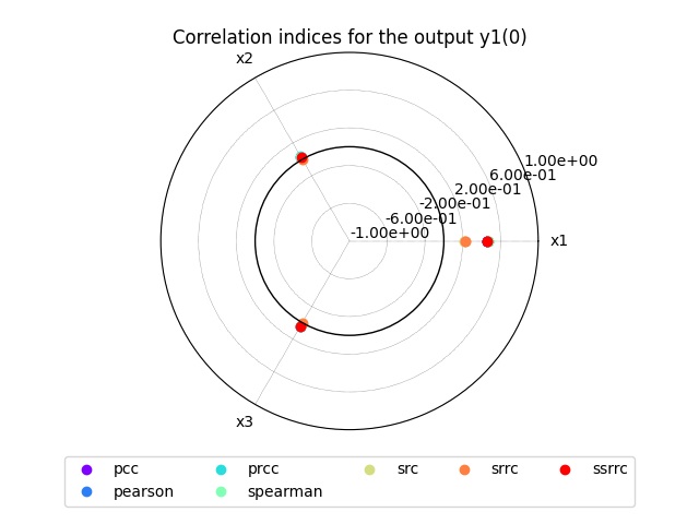
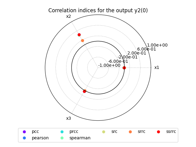
Lastly,
we can use the method CorrelationAnalysis.plot()
to visualize the different correlation coefficients:
correlation.plot("y1", save=False, show=False)
correlation.plot("y2", save=False, show=False)
# Workaround for HTML rendering, instead of ``show=True``
plt.show()
Total running time of the script: ( 0 minutes 1.536 seconds)