Note
Click here to download the full example code
Sobol’ analysis
import pprint

from gemseo.algos.parameter_space import ParameterSpace
from gemseo.api import create_discipline
from gemseo.uncertainty.sensitivity.sobol.analysis import SobolAnalysis
from matplotlib import pyplot as plt
from numpy import pi
In this example, we consider a function from \([-\pi,\pi]^3\) to \(\mathbb{R}^3\):
where \(f(a,b,c)=\sin(a)+7\sin(b)^2+0.1*c^4\sin(a)\) is the Ishigami function:
expressions = {
    "y1": "sin(x1)+7*sin(x2)**2+0.1*x3**4*sin(x1)",
    "y2": "sin(x2)+7*sin(x1)**2+0.1*x3**4*sin(x2)",
}
discipline = create_discipline(
    "AnalyticDiscipline", expressions=expressions, name="Ishigami2"
)
Then, we consider the case where the deterministic variables \(x_1\), \(x_2\) and \(x_3\) are replaced with the uncertain variables \(X_1\), \(X_2\) and \(X_3\). The latter are independent and identically distributed according to an uniform distribution between \(-\pi\) and \(\pi\):
space = ParameterSpace()
for variable in ["x1", "x2", "x3"]:
    space.add_random_variable(
        variable, "OTUniformDistribution", minimum=-pi, maximum=pi
    )
From that,
we would like to carry out a sensitivity analysis with the random outputs
\(Y_1=f(X_1,X_2,X_3)\) and \(Y_2=f(X_2,X_1,X_3)\).
For that,
we can compute the correlation coefficients from a SobolAnalysis:
sobol = SobolAnalysis([discipline], space, 100)
sobol.main_method = "total"
sobol.compute_indices()
Out:
{'first': {'y1': [{'x1': array([0.19426511]),
                   'x2': array([0.21211854]),
                   'x3': array([0.01782884])}],
           'y2': [{'x1': array([0.75387699]),
                   'x2': array([0.26516667]),
                   'x3': array([0.35758815])}]},
 'total': {'y1': [{'x1': array([0.87052721]),
                   'x2': array([0.37726189]),
                   'x3': array([0.29945874])}],
           'y2': [{'x1': array([0.36991381]),
                   'x2': array([0.60974968]),
                   'x3': array([0.34776012])}]}}
The resulting indices are the first and total order Sobol’ indices:
pprint.pprint(sobol.indices)
Out:
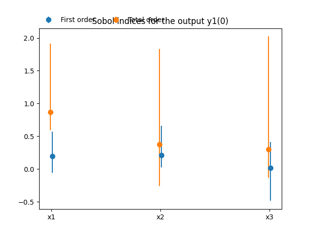
{'first': {'y1': [{'x1': array([0.19426511]),
'x2': array([0.21211854]),
'x3': array([0.01782884])}],
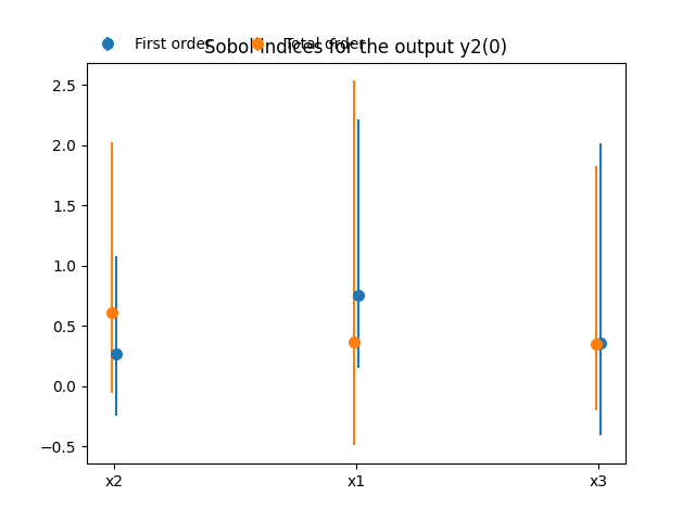
'y2': [{'x1': array([0.75387699]),
'x2': array([0.26516667]),
'x3': array([0.35758815])}]},
'total': {'y1': [{'x1': array([0.87052721]),
'x2': array([0.37726189]),
'x3': array([0.29945874])}],
'y2': [{'x1': array([0.36991381]),
'x2': array([0.60974968]),
'x3': array([0.34776012])}]}}
They can also be accessed separately:
pprint.pprint(sobol.first_order_indices)
pprint.pprint(sobol.total_order_indices)
Out:
{'y1': [{'x1': array([0.19426511]),
         'x2': array([0.21211854]),
         'x3': array([0.01782884])}],
 'y2': [{'x1': array([0.75387699]),
         'x2': array([0.26516667]),
         'x3': array([0.35758815])}]}
{'y1': [{'x1': array([0.87052721]),
         'x2': array([0.37726189]),
         'x3': array([0.29945874])}],
 'y2': [{'x1': array([0.36991381]),
         'x2': array([0.60974968]),
         'x3': array([0.34776012])}]}
The main indices corresponds to the Spearman correlation indices
(this main method can be changed with SobolAnalysis.main_method):
pprint.pprint(sobol.main_indices)

pprint.pprint(sobol.get_intervals())
Out:
{'y1': [{'x1': array([0.87052721]),
         'x2': array([0.37726189]),
         'x3': array([0.29945874])}],
 'y2': [{'x1': array([0.36991381]),
         'x2': array([0.60974968]),
         'x3': array([0.34776012])}]}
{'y1': [{'x1': array([-0.05887176,  0.57198378]),
         'x2': array([0.0281138 , 0.66092945]),
         'x3': array([-0.48592145,  0.41401005])}],
 'y2': [{'x1': array([0.15165848, 2.21224422]),
         'x2': array([-0.24741228,  1.07690768]),
         'x3': array([-0.40957101,  2.01204153])}]}
We can also sort the input parameters by decreasing order of influence: and observe that this ranking is not the same for both outputs:
print(sobol.sort_parameters("y1"))
print(sobol.sort_parameters("y2"))
Out:
['x1', 'x2', 'x3']
['x2', 'x1', 'x3']
Lastly,
we can use the method SobolAnalysis.plot()
to visualize both first and total order Sobol’ indices:
sobol.plot("y1", save=False, show=False)
sobol.plot("y2", save=False, show=False)
# Workaround for HTML rendering, instead of ``show=True``
plt.show()
Total running time of the script: ( 0 minutes 0.410 seconds)