Note
Click here to download the full example code
Fitting a distribution from data based on OpenTURNS
from gemseo.api import configure_logger
from gemseo.uncertainty.distributions.openturns.fitting import OTDistributionFitter
from matplotlib import pyplot as plt
from numpy.random import randn
from numpy.random import seed

configure_logger()
Out:
<RootLogger root (INFO)>
In this example, we will see how to fit a distribution from data. For a purely pedagogical reason, we consider a synthetic dataset made of 100 realizations of ‘X’, a random variable distributed according to the standard normal distribution. These samples are generated from the NumPy library.
seed(1)
data = randn(100)
variable_name = "X"
Create a distribution fitter
Then,
we create an OTDistributionFitter from these data and this variable name:
fitter = OTDistributionFitter(variable_name, data)
Fit a distribution
From this distribution fitter, we can easily fit any distribution available in the OpenTURNS library:
print(fitter.available_distributions)
Out:
['Arcsine', 'Beta', 'Burr', 'Chi', 'ChiSquare', 'Dirichlet', 'Exponential', 'FisherSnedecor', 'Frechet', 'Gamma', 'GeneralizedPareto', 'Gumbel', 'Histogram', 'InverseNormal', 'Laplace', 'LogNormal', 'LogUniform', 'Logistic', 'MeixnerDistribution', 'Normal', 'Pareto', 'Rayleigh', 'Rice', 'Student', 'Trapezoidal', 'Triangular', 'TruncatedNormal', 'Uniform', 'VonMises', 'WeibullMax', 'WeibullMin']
For example, we can fit a normal distribution:
norm_dist = fitter.fit("Normal")
print(norm_dist)
Out:
Normal(class=Point name=Unnamed dimension=2 values=[0.0605829,0.889615])
or an exponential one:
exp_dist = fitter.fit("Exponential")
print(exp_dist)
Out:
Exponential(class=Point name=Unnamed dimension=2 values=[0.419342,-2.3241])
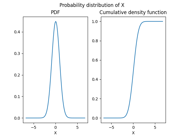
The returned object is an OTDistribution
that we can represent graphically
in terms of probability and cumulative density functions:
norm_dist.plot(show=False)
# Workaround for HTML rendering, instead of ``show=True``
plt.show()
Measure the goodness-of-fit
We can also measure the goodness-of-fit of a distribution by means of a fitting criterion. Some fitting criteria are based on significance tests made of a test statistics, a p-value and a significance level. We can access the names of the available fitting criteria:
print(fitter.available_criteria)
print(fitter.available_significance_tests)
Out:
['BIC', 'ChiSquared', 'Kolmogorov']
['ChiSquared', 'Kolmogorov']
For example, we can measure the goodness-of-fit of the previous distributions by considering the Bayesian information criterion (BIC):
quality_measure = fitter.compute_measure(norm_dist, "BIC")
print("Normal: ", quality_measure)

quality_measure = fitter.compute_measure(exp_dist, "BIC")
print("Exponential: ", quality_measure)
Out:
Normal:  2.5939451287694295
Exponential:  3.7381346286469945
Here, the fitted normal distribution is better than the fitted exponential one in terms of BIC. We can also the Kolmogorov fitting criterion which is based on the Kolmogorov significance test:
acceptable, details = fitter.compute_measure(norm_dist, "Kolmogorov")
print("Normal: ", acceptable, details)
acceptable, details = fitter.compute_measure(exp_dist, "Kolmogorov")
print("Exponential: ", acceptable, details)
Out:
Normal:  True {'p-value': 0.9879299613543082, 'statistics': 0.04330972976650932, 'level': 0.05}
Exponential:  False {'p-value': 5.628454180958696e-11, 'statistics': 0.34248997332293696, 'level': 0.05}
In this case,
the OTDistributionFitter.measure() method returns a tuple with two values:
a boolean indicating if the measured distribution is acceptable to model the data,
a dictionary containing the test statistics, the p-value and the significance level.
Note
We can also change the significance level for significance tests
whose default value is 0.05.
For that, use the level argument.
Select an optimal distribution
Lastly,
we can also select an optimal OTDistribution
based on a collection of distributions names,
a fitting criterion,
a significance level
and a selection criterion:
‘best’: select the distribution minimizing (or maximizing, depending on the criterion) the criterion,
‘first’: select the first distribution for which the criterion is greater (or lower, depending on the criterion) than the level.
By default,
the OTDistributionFitter.select() method uses a significance level equal to 0.5
and ‘best’ selection criterion.
selected_distribution = fitter.select(["Exponential", "Normal"], "Kolmogorov")
print(selected_distribution)
Out:
Normal(class=Point name=Unnamed dimension=2 values=[0.0605829,0.889615])
Total running time of the script: ( 0 minutes 0.158 seconds)