Note
Click here to download the full example code
Probability distributions based on OpenTURNS
In this example, we seek to create a probability distribution based on the OpenTURNS library.
from gemseo.api import configure_logger
from gemseo.uncertainty.api import create_distribution
from gemseo.uncertainty.api import get_available_distributions
from matplotlib import pyplot as plt

configure_logger()
Out:
<RootLogger root (INFO)>
First of all, we can access the names of the available probability distributions from the API:
all_distributions = get_available_distributions()
print(all_distributions)
Out:
['ComposedDistribution', 'OTComposedDistribution', 'OTDiracDistribution', 'OTDistribution', 'OTExponentialDistribution', 'OTNormalDistribution', 'OTTriangularDistribution', 'OTUniformDistribution', 'SPComposedDistribution', 'SPDistribution', 'SPExponentialDistribution', 'SPNormalDistribution', 'SPTriangularDistribution', 'SPUniformDistribution']
and filter the ones based on the OpenTURNS library (their names start with the acronym ‘OT’):
ot_distributions = [dist for dist in all_distributions if dist.startswith("OT")]
print(ot_distributions)
Out:
['OTComposedDistribution', 'OTDiracDistribution', 'OTDistribution', 'OTExponentialDistribution', 'OTNormalDistribution', 'OTTriangularDistribution', 'OTUniformDistribution']
Create a distribution
Then, we can create a probability distribution for a two-dimensional random variable whose components are independent and distributed as the standard normal distribution (mean = 0 and standard deviation = 1):
distribution_0_1 = create_distribution("x", "OTNormalDistribution", 2)
print(distribution_0_1)
Out:
Normal(mu=0.0, sigma=1.0)
or create another distribution with mean = 1 and standard deviation = 2 for the marginal distributions:
distribution_1_2 = create_distribution(
    "x", "OTNormalDistribution", 2, mu=1.0, sigma=2.0
)
print(distribution_1_2)
Out:
Normal(mu=1.0, sigma=2.0)
We could also use the generic OTDistribution
which allows access to all the OpenTURNS distributions
but this requires to know the signature of the methods of this library:
distribution_1_2 = create_distribution(
    "x", "OTDistribution", 2, interfaced_distribution="Normal", parameters=(1.0, 2.0)
)
print(distribution_1_2)
Out:
Normal(1.0, 2.0)
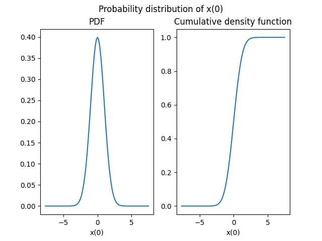
Plot the distribution
We can plot both cumulative and probability density functions for the first marginal:
distribution_0_1.plot(show=False)
# Workaround for HTML rendering, instead of ``show=True``
plt.show()
Note
We can provide a marginal index
as first argument of the Distribution.plot() method
but in the current version of GEMSEO,
all components have the same distributions and so the plot will be the same.
Get mean
We can access the mean of the distribution:
print(distribution_0_1.mean)
Out:
[0. 0.]
Get standard deviation
We can access the standard deviation of the distribution:
print(distribution_0_1.standard_deviation)
Out:
[1. 1.]
Get numerical range
We can access the range, ie. the difference between the numerical minimum and maximum, of the distribution:
print(distribution_0_1.range)
Out:
[array([-7.65062809, 7.65062809]), array([-7.65062809, 7.65062809])]
Get mathematical support
We can access the range, ie. the difference between the minimum and maximum, of the distribution:
print(distribution_0_1.support)
Out:
[array([-inf, inf]), array([-inf, inf])]
Generate samples
We can generate 10 samples of the distribution:
print(distribution_0_1.compute_samples(10))
Out:
[[ 1.43360432 -0.21131498]
 [-0.22736098  0.71315714]
 [-0.38085859  1.09602106]
 [ 0.79766649 -0.20274454]
 [-1.36069266 -0.73384049]
 [-0.9452202  -1.50261139]
 [ 0.86127906  1.07794488]
 [-0.49622029  1.60805988]
 [ 2.10526732  0.25936155]
 [-0.72830578  1.67838523]]
Compute CDF
We can compute the cumulative density function component per component (here the probability that the first component is lower than 0. and that the second one is lower than 1.):
.. GENERATED FROM PYTHON SOURCE LINES 129-131
print(distribution_0_1.compute_cdf([0.0, 1.0]))
Out:
[0.5 0.84134475]
Compute inverse CDF
We can compute the inverse cumulative density function component per component (here the quantile at 50% for the first component and the quantile at 97.5% for the second one):
print(distribution_0_1.compute_inverse_cdf([0.5, 0.975]))
Out:
[0. 1.95996398]
Total running time of the script: ( 0 minutes 0.166 seconds)