Multi Disciplinary Analyses
This section deals with the construction and execution of a Multi Disciplinary Analysis (MDA), i.e. the computation and the convergence of the coupling variables of coupled disciplines.
See also
Examples are given in sobieski_mdo.
Creation of the MDAs
Two families of MDA methods are implemented in GEMSEO
and can be created with the function create_mda():
- fixed-point algorithms,
that compute fixed points of a coupling function \(y\), that is they solve the system \(y(x) = x\)
- Newton method algorithms for root finding,
that solve a non-linear multivariate problem \(R(x, y) = 0\) using the derivatives \(\frac{\partial R(x, y)}{\partial y} = 0\) where \(R(x, y)\) is the residual.
Any explicit problem of the form \(y(x) = x\) can be reformulated into a root finding problem by stating \(R(x, y) = y(x) - x = 0\). The opposite is not true. This means that if the disciplines are provided in a residual form, the Gauss-Seidel algorithm for instance cannot be directly used.
Warning
Any MDODiscipline placed in an MDA
with strong couplings must define its default inputs.
Otherwise, the execution will fail.
Fixed-point algorithms
Fixed-point algorithms include Gauss-Seidel algorithm and Jacobi algorithms.
from gemseo.api import create_mda, create_discipline

disciplines = create_discipline(["SobieskiPropulsion", "SobieskiAerodynamics",
                                "SobieskiMission", "SobieskiStructure"])

mda_gaussseidel = create_mda("MDAGaussSeidel", disciplines)
mda_jacobi = create_mda("MDAJacobi", disciplines)
See also
The classes MDAGaussSeidel
and MDAJacobi
called by create_mda(),
inherit from MDA,
itself inheriting from MDODiscipline.
Therefore,
an MDA based on a fixed-point algorithm can be viewed as a discipline
whose inputs are design variables and outputs are coupling variables.
Root finding methods
Newton-Raphson method
The Newton-Raphson method is parameterized by a relaxation factor \(\alpha \in (0, 1]\) to limit the length of the steps taken along the Newton direction. The new iterate is given by: \(x_{k+1} = x_k - \alpha f'(x_k)^{-1} f(x_k)\).
mda = create_mda("MDANewtonRaphson", disciplines, relax_factor=0.99)
Quasi-Newton method
Quasi-Newton methods
include numerous variants (Broyden,
Levenberg-Marquardt, …).
The name of the variant should be provided with the argument method.
mda = create_mda("MDAQuasiNewton", disciplines, method=MDAQuasiNewton.BROYDEN1)
See also
The classes MDANewtonRaphson
and MDAQuasiNewton
called by create_mda(),
inherit from MDARoot,
itself inheriting from MDA,
itself inheriting from MDODiscipline.
Therefore,
an MDA based on a root finding method can be viewed as a discipline
whose inputs are design variables and outputs are coupling variables.
Hybrid methods
Hybrid methods implement a generic scheme to combine elementary MDAs:
an arbitrary number of them are provided and are executed sequentially.
The following code creates a hybrid mda that runs sequentially
one iteration of Jacobi method mda1
and a full Newton-Raphson method mda2.
mda1 = create_mda("MDAJacobi", disciplines, max_mda_iter=1)
mda2 = create_mda("MDANewtonRaphson", disciplines)
mda = create_mda("MDASequential", disciplines, mda_sequence = [mda1, mda2])
This sequence is typically used to take advantage of the robustness of fixed-point methods and then obtain accurate results thanks to a Newton method.
Execution and convergence analysis
The MDAs are run using the default input data
of the disciplines as a starting point.
A MDA provides a method to plot the evolution
of the residuals of the system with respect to the iterations ;
the plot may be displayed and/or saved with
plot_residual_history():
mda.plot_residual_history(n_iterations=10, logscale=[1e-8, 10.])
The next plots compare the convergence of
Gauss-Seidel, Jacobi, quasi-Newton and the hybrid
with respect to the iterations.
Identical scales were used for the plots
(n_iterations for the \(x\) axis and logscale for the
logarithmic \(y\) axis, respectively).
It shows that,
as expected,
Gauss-Seidel has a better convergence than the Jacobi method.
The hybrid MDA,
combining an iteration of Gauss-Seidel and a full Quasi-Newton,
converges must faster than all the other alternatives ;
note that Newton-Raphson alone does not converge well
for the initial values of the coupling variables.
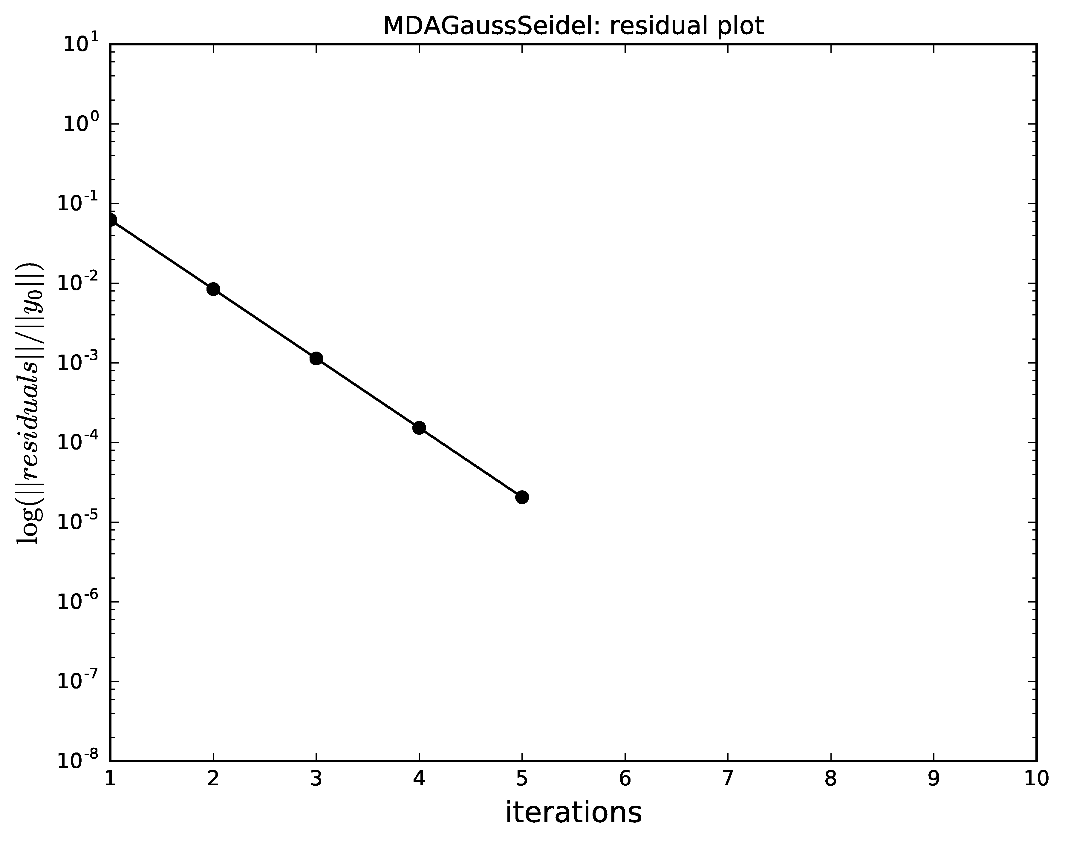
Gauss-Seidel algorithm convergence for MDA.
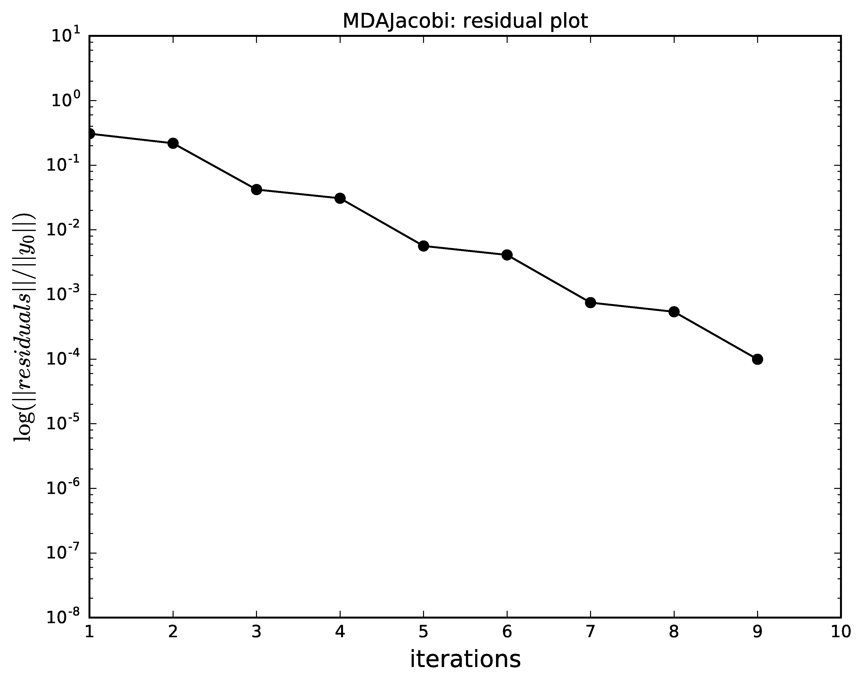
Jacobi algorithm convergence for MDA.
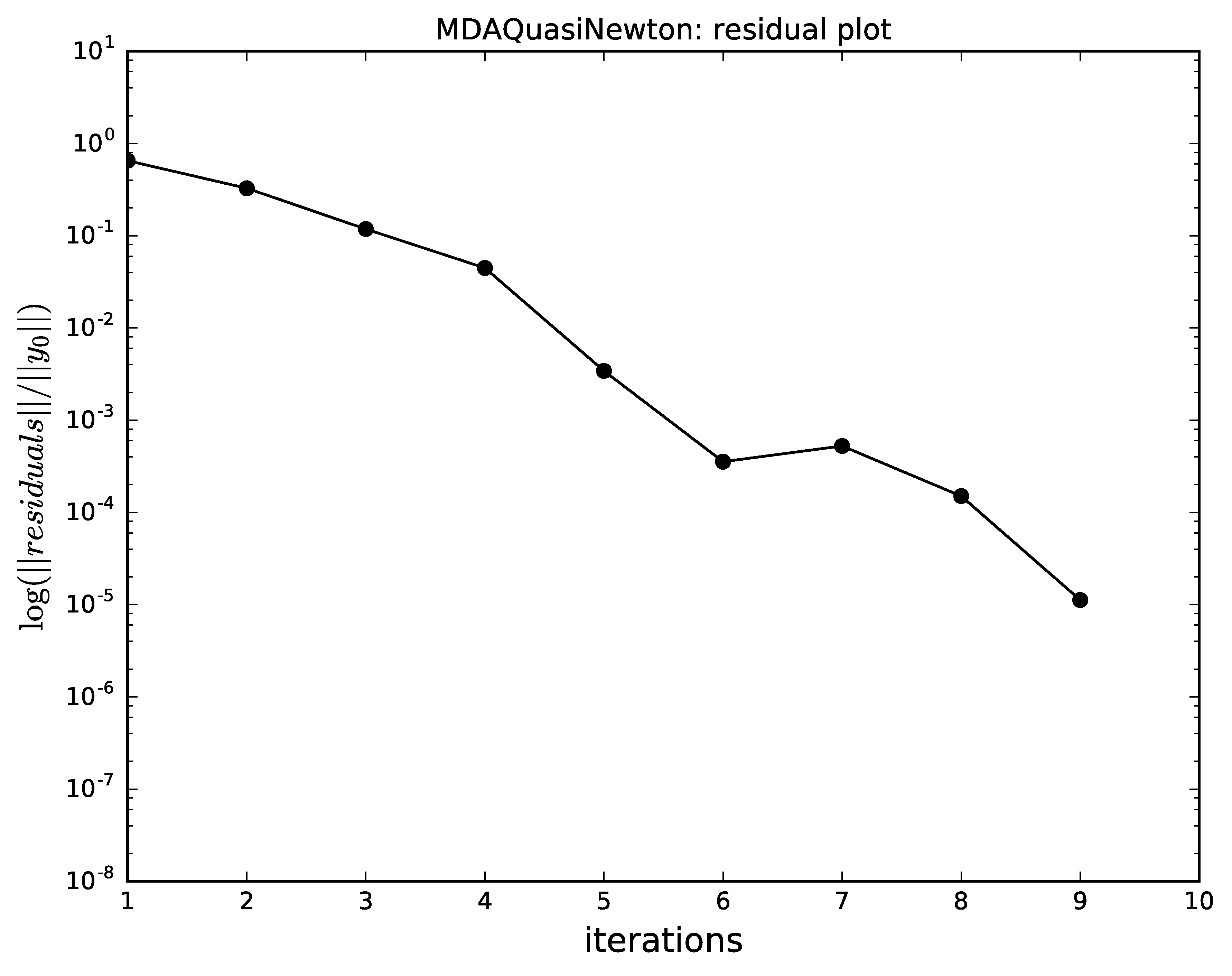
Quasi-Newton algorithm convergence for MDA.
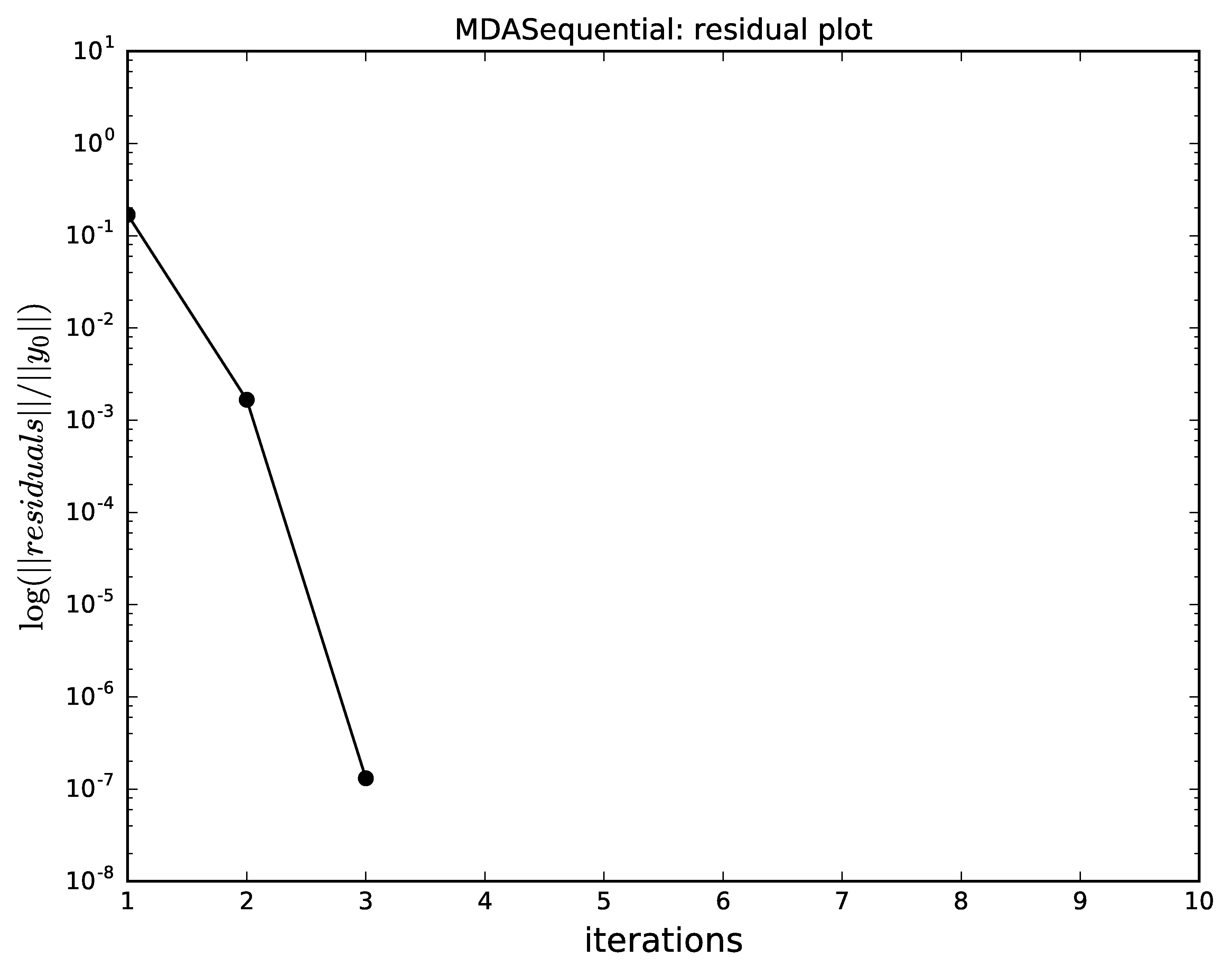
Hybrid Gauss-Seidel and a Quasi-Newton algorithm convergence for MDA.
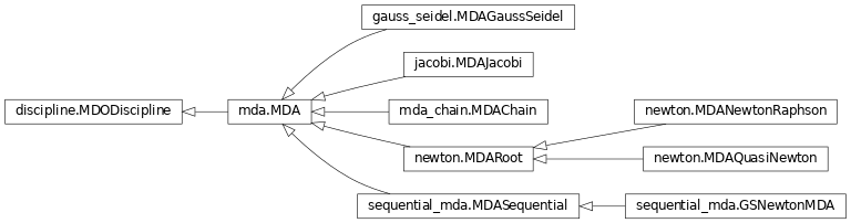
Classes organization
The following inheritance diagram shows the different MDA classes in GEMSEO and their organization.
MDAChain and the Coupling structure for smart MDAs
The MDOCouplingStructure
provides methods to compute the coupling variables between the disciplines:
from gemseo.core.coupling_structure import MDOCouplingStructure

coupling_structure = MDOCouplingStructure(disciplines)
This is an internal object that is created in all MDA classes and all formulations. The end user does not need to create it for basic usage.
The MDOCouplingStructure
uses graphs to compute the dependencies between the disciplines,
and therefore the coupling variables.
This graph can then be used to generate a process
to solve the coupling problem with a coupling algorithm.
To illustrate the typical procedure, we take a dummy 16 disciplines problem.
First the coupling graph is generated.
Then, a minimal process is computed, with eventually inner-MDAs. A set of coupling problems is generated, which are passed to algorithms.
Finally, a Jacobi MDA is used to solve the coupling equations, via the SciPy package, or directly coded in GEMSEO (Gauss-Seidel and Jacobi for instance). They can be compared on the specific problem, and MDAs can generate convergence plots of the residuals.
The next figure illustrates this typical process
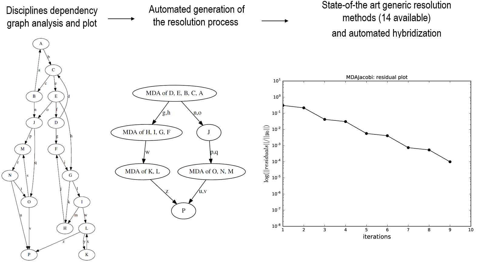
The 3 resolution phases of a 16 disciplines coupling problem
This features is used in the MDAChain
which generates a chain of MDAs according
to the graph of dependency in order to minimize the execution time.
The user provides a base MDA class to solve the coupled problems.
The overall sequential process made of inner-MDAs and
disciplines execution is created by a MDOChain.
The inner-MDAs can be specified using the argument inner_mda_name.
mda = create_mda("MDAChain", disciplines, inner_mda_name="MDAJacobi")
mda.execute()