Benchmark problems
In this section, we describe the GEMSEO’s benchmark MDO problems:
Sellar’s problem
The Sellar’s problem is considered in different tutorials:
Description of the problem
The Sellar problem is defined by analytical functions:
where the coupling variables are
and
and where the general constraints are
The Sellar disciplines are also available with analytic derivatives in GEMSEO, as well as a DesignSpace:
Creation of the disciplines
To create the Sellar disciplines, use the function create_discipline:
from gemseo.api import create_discipline

disciplines = create_discipline(["Sellar1", "Sellar2", "SellarSystem"])
Importation of the design space
To import the Sellar design space, use the class create_discipline:
from gemseo.problems.sellar.sellar_design_space import SellarDesignSpace
design_space = SellarDesignSpace()
Then, you can visualize it with print(design_space):
+----------+-------------+--------+-------------+-------+
| name     | lower_bound | value  | upper_bound | type  |
+----------+-------------+--------+-------------+-------+
| x_local  |      0      | (1+0j) |      10     | float |
+          +             +        +             +       +
| x_shared |     -10     | (4+0j) |      10     | float |
+          +             +        +             +       +
| x_shared |      0      | (3+0j) |      10     | float |
+          +             +        +             +       +
| y_1      |     -100    | (1+0j) |     100     | float |
+          +             +        +             +       +
| y_2      |     -100    | (1+0j) |     100     | float |
+----------+-------------+--------+-------------+-------+
See also
See Tutorial: How to solve an MDO problem to create the Sellar problem from scratch
Aerostructure problem
The Sobieski’s SSBJ test case is considered in the different tutorials:
Description of the problem
The Aerostructure problem is defined by analytical functions:
where
and
where
and
The Aerostructure disciplines are also available with analytic derivatives in the classes Mission, Aerodynamics and Structure, as well as a AerostructureDesignSpace:
Creation of the disciplines
To create the aerostructure disciplines, use the function create_discipline():
from gemseo.api import create_discipline

disciplines = create_discipline(["Aerodynamics",
                                 "Structure",
                                 "Mission"])
Importation of the design space
To import the aerostructure design space, use the class create_discipline:
from gemseo.problems.aerostructure.aerostructure_design_space import AerostructureDesignSpace
design_space = AerostructureDesignSpace()
Then, you can visualize it with print(design_space):
+----------------+-------------+-------------+-------------+-------+
| name           | lower_bound |    value    | upper_bound | type  |
+----------------+-------------+-------------+-------------+-------+
| thick_airfoils |      5      |   (15+0j)   |      25     | float |
| thick_panels   |      1      |    (3+0j)   |      20     | float |
| sweep          |      10     |   (25+0j)   |      35     | float |
| drag           |     100     |   (340+0j)  |     1000    | float |
| forces         |    -1000    |   (400+0j)  |     1000    | float |
| lift           |     0.1     |   (0.5+0j)  |      1      | float |
| mass           |    100000   | (100000+0j) |    500000   | float |
| displ          |    -1000    |  (-700+0j)  |     1000    | float |
| rf             |    -1000    |      0j     |     1000    | float |
+----------------+-------------+-------------+-------------+-------+
See also
See MDO formulations and scalable models for a toy example in aerostructure to see an application of this problem.
Sobieski’s SSBJ test case
The Sobieski’s SSBJ test case is considered in the different tutorials:
Origin of the test case
This test was taken from the reference article by Sobieski, the first publication on the BLISS formulation. It is based on a 1996 AIAA student competition organized by the AIAA/United Technologies/Pratt & Whitney Individual Undergraduate Design Competition. This competition initially focused on both the technical and economical challenges of a development.
The formulas used for each are based on semi-empirical and/or analytical models. Depending on the , some examples can be found in the following references [Niu88][And36][Ray06]. As specified by Sobieski et al., additional design and state variables (not present in the original problem) were introduced in the disciplinary analyses for testing purposes.
The MDO problem
The aim of the problem is to maximize the range of a Super-Sonic Business under various constraints.
The problem is built from three disciplines: structure, aerodynamics and propulsion.
A fourth discipline, not coupled to the other ones, is required to compute the range.
Input and output variables
The next tables display the input variables required by each of the four disciplines.
As they are shared by several disciplines, global design variables, implemented as \(x\_shared\), are provided to all disciplines.
Coupling variables are implemented as \(y\_ij\), which is an output of discipline \(i\) and an input of discipline \(j\).
Disciplines are listed as follows
Structure,
Aerodynamics,
Propulsion,
Range.
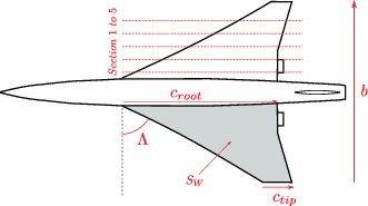
The SSBJ planform variables
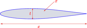
The airfoils variables
Variable |
Description |
Bounds |
Symbol |
|---|---|---|---|
\(t/c\) |
Thickness to chord ratio |
\(0.01\leq t/c\leq 0.09\) |
\(x\_shared[0]\) |
\(h\) |
Altitude (\(ft\)) |
\(30000\leq h \leq 60000\) |
\(x\_shared[1]\) |
\(M\) |
Mach number |
\(1.4\leq M\leq 1.8\) |
\(x\_shared[2]\) |
\(AR=b^2/S_W\) |
Aspect ratio |
\(2.5\leq AR\leq 8.5\) |
\(x\_shared[3]\) |
\(\Lambda\) |
Wing sweep (\(\deg\)) |
\(40\leq\Lambda\leq70\) |
\(x\_shared[4]\) |
\(S_W\) |
Wing surface area (\(ft^2\)) |
\(500\leq S\leq 1500\) |
\(x\_shared[5]\) |
\(\lambda = {c_{tip}}/{c_{root}}\) |
Wing taper ratio |
\(0.1\leq\lambda\leq0.4\) |
\(x\_1[0]\) |
\(x\) |
Wingbox x-sectional area |
\(0.75\leq x \leq 1.25\) |
\(x\_1[1]\) |
\(L\) |
Lift from aerodynamics (\(N\)) |
\(y\_21[0]\) |
|
\(W_{E}\) |
Engine mass from propulsion (\(lb\)) |
\(y\_31[0]\) |
|
\(C_f\) |
Skin friction coefficient |
\(0.75\leq Cf\leq 1.25\) |
\(x\_2[0]\) |
\(W_T\) |
Total aircraft mass from structure |
\(y\_12[0]\) |
|
\(\Delta\alpha_v\) |
Wing twist from structure |
\(y\_12[1]\) |
|
\(ESF\) |
Engine scale factor from propulsion |
\(y\_32[0]\) |
|
\(Th\) |
Throttle setting (engine mass flow) |
\(0.1\leq T\leq 1.25\) |
\(x\_3[0]\) |
\(D\) |
Drag from aerodynamics (\(N\)) |
\(y\_23[0]\) |
|
\(L/D\) |
Lift-over-drag ratio from aerodynamics |
\(y\_24[0]\) |
|
\(W_T\) |
Total aircraft mass from structure |
\(y\_14[0]\) |
|
\(W_F\) |
Fuel mass from structure |
\(y\_14[1]\) |
|
\(SFC\) |
Specific Fuel Consumption from propulsion |
\(y\_34[0]\) |
Table: Input variables of Sobieski’s problem
Variable |
Description |
Constraint |
Symbol |
|---|---|---|---|
\(\sigma_1\) |
Stress constraints on wing section 1 |
\(\sigma_1<1.09\) |
\(g\_1[0]\) |
\(\sigma_2\) |
Stress constraints on wing section 2 |
\(\sigma_2<1.09\) |
\(g\_1[1]\) |
\(\sigma_3\) |
Stress constraints on wing section 3 |
\(\sigma_3<1.09\) |
\(g\_1[2]\) |
\(\sigma_4\) |
Stress constraints on wing section 4 |
\(\sigma_4<1.09\) |
\(g\_1[3]\) |
\(\sigma_5\) |
Stress constraints on wing section 5 |
\(\sigma_5<1.09\) |
\(g\_1[4]\) |
\(W_T\) |
Total aircraft mass (\(lb\)) |
\(y\_1[0]\) |
|
\(W_F\) |
Fuel mass (\(lb\)) |
\(y\_1[1]\) |
|
\(\Delta\alpha_{v}\) |
Wing twist (\(\deg\)) |
\(0.96<\Delta\alpha_{v}<1.04\) |
\(y\_1[2],g_1[5]\) |
\(L\) |
Lift (\(N\)) |
\(y\_2[0]\) |
|
\(D\) |
Drag (\(N\)) |
\(y\_2[1]\) |
|
\(L/D\) |
Lift-over-drag ratio |
\(y\_2[2]\) |
|
\(dp/dx\) |
Pressure gradient |
\(dp/dx<1.04\) |
\(g\_2[0]\) |
\(SFC\) |
Specific Fuel Consumption |
\(y\_3[0]\) |
|
\(W_E\) |
Engine mass (\(lb\)) |
\(y\_3[1]\) |
|
\(ESF\) |
Engine Scale Factor |
\(0.5\leq ESF \leq 1.5\) |
\(y\_3[2],g_3[0]\) |
\(T_E\) |
Engine temperature |
\(T_E\leq 1.02\) |
\(g\_3[1]\) |
\(Th\) |
Throttle setting constraint |
\(Th\leq Th_{uA}\) |
\(g\_3[2]\) |
\(R\) |
Range (\(nm\)) |
\(y\_4[0]\) |
Table: Output variables of Sobieski’s problem
Creation of the disciplines
To create the SSBJ disciplines :
from gemseo.api import  create_discipline

disciplines = create_discipline(["SobieskiStructure",
                                "SobieskiPropulsion",
                                "SobieskiAerodynamics",
                                "SobieskiMission"])
Reference results
This problem was implemented by Sobieski et al. in Matlab and Isight. Both implementations led to the same results.
As all gradients can be computed, we resort to gradient-based optimization methods. All Jacobian matrices are coded analytically in GEMSEO.
Reference results using the MDF formulation are presented in the next table.
Variable |
Initial |
Optimum |
|---|---|---|
Range (nm) |
535.79 |
3963.88 |
\(\lambda\) |
0.25 |
0.38757 |
\(x\) |
1 |
0.75 |
\(C_f\) |
1 |
0.75 |
\(Th\) |
0.5 |
0.15624 |
\(t/c\) |
0.05 |
0.06 |
\(h\) \((ft)\)) |
45000 |
60000 |
\(M\) |
1.6 |
1.4 |
\(AR\) |
5.5 |
2.5 |
\(\Lambda\) \((\deg)\) |
55 |
70 |
\(S_W\) \((ft^2)\) |
1000 |
1500 |
The Propane combustion problem
The Propane MDO problem can be found in [PAG96] and [TM06]. It represents the chemical equilibrium reached during the combustion of propane in air. Variables are assigned to represent each of the ten combustion products as well as the sum of the products.
The optimization problem is as follows:
where the System Discipline consists of computing the following expressions:
Discipline 1 computes \((x_{2}, x_{4})\) by satisfying the following equations:
Discipline 2 computes \((x_2, x_4)\) such that:
and Discipline 3 computes \((x_5, x_9, x_{11})\) by solving:
Creation of the disciplines
The Propane combustion disciplines are available in GEMSEO and can be imported with the following code:
from gemseo.api import  create_discipline

disciplines = create_discipline(["PropaneComb1",
                                "PropaneComb2",
                                "PropaneComb3",
                                "PropaneReaction"])
A gemseo.algos.design_space.DesignSpace file propane_design_space.txt is also available in the same folder, which can be read using
the gemseo.api.read_design_space() method.
Problem results
The optimum is \((x1,x3,x6,x7) = (1.378887, 18.426810, 1.094798, 0.931214)\). The minimum objective value is \(0\). At this point, all the system-level inequality constraints are active.