Correlation analysis

from __future__ import annotations

import pprint

from gemseo.uncertainty.sensitivity.correlation.analysis import CorrelationAnalysis
from gemseo.uncertainty.use_cases.ishigami.ishigami_discipline import IshigamiDiscipline
from gemseo.uncertainty.use_cases.ishigami.ishigami_space import IshigamiSpace

In this example, we consider the Ishigami function [IH90]

\[f(x_1,x_2,x_3)=\sin(x_1)+7\sin(x_2)^2+0.1x_3^4\sin(x_1)\]

implemented as an MDODiscipline by the IshigamiDiscipline. It is commonly used with the independent random variables \(X_1\), \(X_2\) and \(X_3\) uniformly distributed between \(-\pi\) and \(\pi\) and defined in the IshigamiSpace.

discipline = IshigamiDiscipline()
uncertain_space = IshigamiSpace()

Then, we run sensitivity analysis of type CorrelationAnalysis:

sensitivity_analysis = CorrelationAnalysis([discipline], uncertain_space, 1000)
sensitivity_analysis.compute_indices()

{<Method.KENDALL: 'Kendall'>: {'y': [{'x1': array([0.31460661]), 'x2': array([0.02366366]), 'x3': array([0.0297978])}]}, <Method.PCC: 'PCC'>: {'y': [{'x1': array([0.46282123]), 'x2': array([0.0306214]), 'x3': array([0.0512473])}]}, <Method.PEARSON: 'Pearson'>: {'y': [{'x1': array([0.46230446]), 'x2': array([0.02059071]), 'x3': array([0.04979026])}]}, <Method.PRCC: 'PRCC'>: {'y': [{'x1': array([0.47248718]), 'x2': array([0.04368652]), 'x3': array([0.0419606])}]}, <Method.SPEARMAN: 'Spearman'>: {'y': [{'x1': array([0.47177886]), 'x2': array([0.03220921]), 'x3': array([0.04128518])}]}, <Method.SRC: 'SRC'>: {'y': [{'x1': array([0.46220697]), 'x2': array([0.027121]), 'x3': array([0.04542585])}]}, <Method.SRRC: 'SRRC'>: {'y': [{'x1': array([0.4718925]), 'x2': array([0.03849088]), 'x3': array([0.03696642])}]}, <Method.SSRC: 'SSRC'>: {'y': [{'x1': array([0.21363529]), 'x2': array([0.00073555]), 'x3': array([0.00206351])}]}}

The resulting indices are

• the Pearson correlation coefficients,

• the Spearman correlation coefficients,

• the Partial Correlation Coefficients (PCC),

• the Partial Rank Correlation Coefficients (PRCC),

• the Standard Regression Coefficients (SRC),

• the Standard Rank Regression Coefficient (SRRC),

• the Signed Standard Rank Regression Coefficient (SSRRC):

pprint.pprint(sensitivity_analysis.indices)

{<Method.KENDALL: 'Kendall'>: {'y': [{'x1': array([0.31460661]),
                                      'x2': array([0.02366366]),
                                      'x3': array([0.0297978])}]},
 <Method.PCC: 'PCC'>: {'y': [{'x1': array([0.46282123]),
                              'x2': array([0.0306214]),
                              'x3': array([0.0512473])}]},
 <Method.PRCC: 'PRCC'>: {'y': [{'x1': array([0.47248718]),
                                'x2': array([0.04368652]),
                                'x3': array([0.0419606])}]},
 <Method.PEARSON: 'Pearson'>: {'y': [{'x1': array([0.46230446]),
                                      'x2': array([0.02059071]),
                                      'x3': array([0.04979026])}]},
 <Method.SRC: 'SRC'>: {'y': [{'x1': array([0.46220697]),
                              'x2': array([0.027121]),
                              'x3': array([0.04542585])}]},
 <Method.SRRC: 'SRRC'>: {'y': [{'x1': array([0.4718925]),
                                'x2': array([0.03849088]),
                                'x3': array([0.03696642])}]},
 <Method.SSRC: 'SSRC'>: {'y': [{'x1': array([0.21363529]),
                                'x2': array([0.00073555]),
                                'x3': array([0.00206351])}]},
 <Method.SPEARMAN: 'Spearman'>: {'y': [{'x1': array([0.47177886]),
                                        'x2': array([0.03220921]),
                                        'x3': array([0.04128518])}]}}

The main indices corresponds to the Spearman correlation indices (this main method can be changed with CorrelationAnalysis.main_method):

pprint.pprint(sensitivity_analysis.main_indices)

{'y': [{'x1': array([0.47177886]),
        'x2': array([0.03220921]),
        'x3': array([0.04128518])}]}

We can also get the input parameters sorted by decreasing order of influence:

sensitivity_analysis.sort_parameters("y")

['x1', 'x3', 'x2']

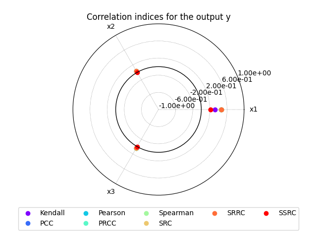
We can use the method CorrelationAnalysis.plot() to visualize the different correlation coefficients:

sensitivity_analysis.plot("y", save=False, show=True)

Lastly, the sensitivity indices can be exported to a Dataset:

sensitivity_analysis.to_dataset()

GROUP	Kendall	PCC	Pearson	PRCC	Spearman	SRC	SRRC	SSRC
VARIABLE	y	y	y	y	y	y	y	y
COMPONENT	0	0	0	0	0	0	0	0
x1	0.314607	0.462821	0.462304	0.472487	0.471779	0.462207	0.471893	0.213635
x2	0.023664	0.030621	0.020591	0.043687	0.032209	0.027121	0.038491	0.000736
x3	0.029798	0.051247	0.049790	0.041961	0.041285	0.045426	0.036966	0.002064