Morris analysis

from __future__ import annotations

import pprint

from gemseo.uncertainty.sensitivity.morris.analysis import MorrisAnalysis
from gemseo.uncertainty.use_cases.ishigami.ishigami_discipline import IshigamiDiscipline
from gemseo.uncertainty.use_cases.ishigami.ishigami_space import IshigamiSpace

In this example, we consider the Ishigami function [IH90]

\[f(x_1,x_2,x_3)=\sin(x_1)+7\sin(x_2)^2+0.1x_3^4\sin(x_1)\]

implemented as an MDODiscipline by the IshigamiDiscipline. It is commonly used with the independent random variables \(X_1\), \(X_2\) and \(X_3\) uniformly distributed between \(-\pi\) and \(\pi\) and defined in the IshigamiSpace.

discipline = IshigamiDiscipline()
uncertain_space = IshigamiSpace()

Then, we run sensitivity analysis of type MorrisAnalysis:

sensitivity_analysis = MorrisAnalysis([discipline], uncertain_space, 10)
sensitivity_analysis.compute_indices()

{'MU': {'y': [{'x1': array([0.73532408]), 'x2': array([-0.05115399]), 'x3': array([-1.6024484])}]}, 'MU_STAR': {'y': [{'x1': array([0.76770333]), 'x2': array([2.09435091]), 'x3': array([1.6024484])}]}, 'SIGMA': {'y': [{'x1': array([0.76770333]), 'x2': array([2.09435091]), 'x3': array([1.58984353])}]}, 'RELATIVE_SIGMA': {'y': [{'x1': array([1.]), 'x2': array([1.]), 'x3': array([0.99213399])}]}, 'MIN': {'y': [{'x1': array([0.03237925]), 'x2': array([2.04319692]), 'x3': array([0.01260487])}]}, 'MAX': {'y': [{'x1': array([1.50302741]), 'x2': array([2.14550491]), 'x3': array([3.19229192])}]}}

The resulting indices are the empirical means and the standard deviations of the absolute output variations due to input changes.

pprint.pprint(sensitivity_analysis.indices)

{'MAX': {'y': [{'x1': array([1.50302741]),
                'x2': array([2.14550491]),
                'x3': array([3.19229192])}]},
 'MIN': {'y': [{'x1': array([0.03237925]),
                'x2': array([2.04319692]),
                'x3': array([0.01260487])}]},
 'MU': {'y': [{'x1': array([0.73532408]),
               'x2': array([-0.05115399]),
               'x3': array([-1.6024484])}]},
 'MU_STAR': {'y': [{'x1': array([0.76770333]),
                    'x2': array([2.09435091]),
                    'x3': array([1.6024484])}]},
 'RELATIVE_SIGMA': {'y': [{'x1': array([1.]),
                           'x2': array([1.]),
                           'x3': array([0.99213399])}]},
 'SIGMA': {'y': [{'x1': array([0.76770333]),
                  'x2': array([2.09435091]),
                  'x3': array([1.58984353])}]}}

The main indices corresponds to these empirical means (this main method can be changed with MorrisAnalysis.main_method):

pprint.pprint(sensitivity_analysis.main_indices)

{'y': [{'x1': array([0.76770333]),
        'x2': array([2.09435091]),
        'x3': array([1.6024484])}]}

and can be interpreted with respect to the empirical bounds of the outputs:

pprint.pprint(sensitivity_analysis.outputs_bounds)

{'y': [array([0.3861887]), array([14.38383568])]}

We can also get the input parameters sorted by decreasing order of influence:

sensitivity_analysis.sort_parameters("y")

['x2', 'x3', 'x1']

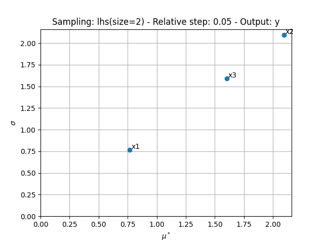
We can use the method MorrisAnalysis.plot() to visualize the different series of indices:

sensitivity_analysis.plot("y", save=False, show=True, lower_mu=0, lower_sigma=0)

Lastly, the sensitivity indices can be exported to a Dataset:

sensitivity_analysis.to_dataset()

GROUP	MU	MU_STAR	SIGMA	RELATIVE_SIGMA	MIN	MAX
VARIABLE	y	y	y	y	y	y
COMPONENT	0	0	0	0	0	0
x1	0.735324	0.767703	0.767703	1.000000	0.032379	1.503027
x2	-0.051154	2.094351	2.094351	1.000000	2.043197	2.145505
x3	-1.602448	1.602448	1.589844	0.992134	0.012605	3.192292