RMSE for regression models

from matplotlib import pyplot as plt
from numpy import array
from numpy import linspace
from numpy import newaxis
from numpy import sin

from gemseo.datasets.io_dataset import IODataset
from gemseo.mlearning.quality_measures.rmse_measure import RMSEMeasure
from gemseo.mlearning.regression.polyreg import PolynomialRegressor
from gemseo.mlearning.regression.rbf import RBFRegressor

Given a dataset \((x_i,y_i,\hat{y}_i)_{1\leq i \leq N}\) where \(x_i\) is an input point, \(y_i\) is an output observation and \(\hat{y}_i=\hat{f}(x_i)\) is an output prediction computed by a regression model \(\hat{f}\), the root mean squared error (RMSE) metric is written

\[\text{RMSE} = \sqrt{\frac{1}{N}\sum_{i=1}^N(y_i-\hat{y}_i)^2} \geq 0.\]

The lower, the better. From a quantitative point of view, this depends on the order of magnitude of the outputs.

To illustrate this quality measure, let us consider the function \(f(x)=(6x-2)^2\sin(12x-4)\) [FSK08]:

def f(x):
    return (6 * x - 2) ** 2 * sin(12 * x - 4)

and try to approximate it with a polynomial of order 3.

For this, we can take these 7 learning input points

x_train = array([0.1, 0.3, 0.5, 0.6, 0.8, 0.9, 0.95])

and evaluate the model f over this design of experiments (DOE):

y_train = f(x_train)

Then, we create an IODataset from these 7 learning samples:

dataset_train = IODataset()
dataset_train.add_input_group(x_train[:, newaxis], ["x"])
dataset_train.add_output_group(y_train[:, newaxis], ["y"])

and build a PolynomialRegressor with degree=3 from it:

polynomial = PolynomialRegressor(dataset_train, 3)
polynomial.learn()

Before using it, we are going to measure its quality with the RMSE metric:

rmse = RMSEMeasure(polynomial)
result = rmse.compute_learning_measure()
result, result / (y_train.max() - y_train.min())

(array([2.37578236]), array([0.137707]))

This result is medium (14% of the learning output range), and we can be expected to a poor generalization quality. As the cost of this academic function is zero, we can approximate this generalization quality with a large test dataset whereas the usual test size is about 20% of the training size.

x_test = linspace(0.0, 1.0, 100)
y_test = f(x_test)
dataset_test = IODataset()
dataset_test.add_input_group(x_test[:, newaxis], ["x"])
dataset_test.add_output_group(y_test[:, newaxis], ["y"])
result = rmse.compute_test_measure(dataset_test)
result, result / (y_test.max() - y_test.min())

(array([3.31730517]), array([0.15181886]))

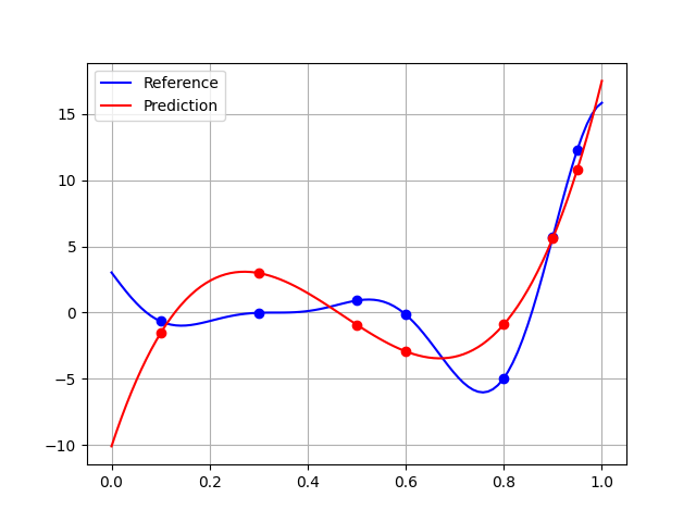
The quality is higher than 15% of the test output range, which is pretty mediocre. This can be explained by a broader generalization domain than that of learning, which highlights the difficulties of extrapolation:

plt.plot(x_test, y_test, "-b", label="Reference")
plt.plot(x_train, y_train, "ob")
plt.plot(x_test, polynomial.predict(x_test[:, newaxis]), "-r", label="Prediction")
plt.plot(x_train, polynomial.predict(x_train[:, newaxis]), "or")
plt.legend()
plt.grid()
plt.show()

Using the learning domain would slightly improve the quality:

x_test = linspace(x_train.min(), x_train.max(), 100)
y_test_in_large_domain = y_test
y_test = f(x_test)
dataset_test_in_learning_domain = IODataset()
dataset_test_in_learning_domain.add_input_group(x_test[:, newaxis], ["x"])
dataset_test_in_learning_domain.add_output_group(y_test[:, newaxis], ["y"])
result = rmse.compute_test_measure(dataset_test_in_learning_domain)
result, result / (y_test.max() - y_test.min())

(array([2.39937613]), array([0.13099891]))

Lastly, to get better results without new learning points, we would have to change the regression model:

rbf = RBFRegressor(dataset_train)
rbf.learn()

The quality of this RBFRegressor is quite good, both on the learning side:

rmse_rbf = RMSEMeasure(rbf)
result = rmse_rbf.compute_learning_measure()
result, result / (y_train.max() - y_train.min())

(array([1.22756756e-14]), array([7.11532547e-16]))

and on the validation side:

result = rmse_rbf.compute_test_measure(dataset_test_in_learning_domain)
result, result / (y_test.max() - y_test.min())

(array([0.14923751]), array([0.00814793]))

including the larger domain:

result = rmse_rbf.compute_test_measure(dataset_test)
result, result / (y_test_in_large_domain.max() - y_test_in_large_domain.min())

(array([0.54182176]), array([0.02479686]))

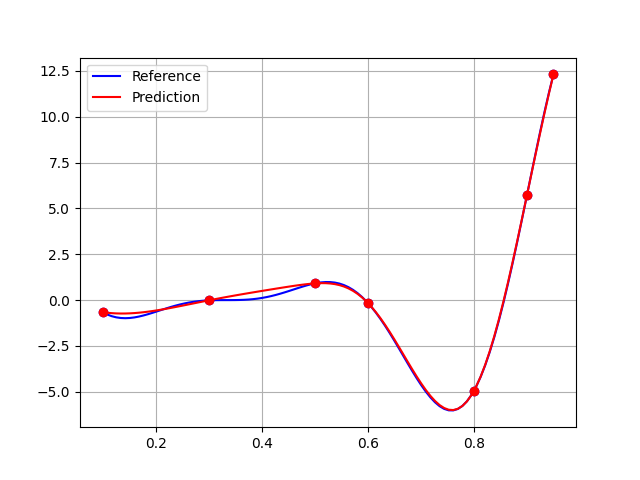
A final plot to convince us:

plt.plot(x_test, y_test, "-b", label="Reference")
plt.plot(x_train, y_train, "ob")
plt.plot(x_test, rbf.predict(x_test[:, newaxis]), "-r", label="Prediction")
plt.plot(x_train, rbf.predict(x_train[:, newaxis]), "or")
plt.legend()
plt.grid()
plt.show()