Note
Go to the end to download the full example code.
MDF-based MDO on the Sobieski SSBJ test case.#
from __future__ import annotations

from gemseo import create_discipline
from gemseo import create_scenario
from gemseo import generate_n2_plot
from gemseo.problems.mdo.sobieski.core.design_space import SobieskiDesignSpace
Instantiate the disciplines#
First, we instantiate the four disciplines of the use case:
SobieskiPropulsion,
SobieskiAerodynamics,
SobieskiMission
and SobieskiStructure.
disciplines = create_discipline([
    "SobieskiPropulsion",
    "SobieskiAerodynamics",
    "SobieskiMission",
    "SobieskiStructure",
])
We can quickly access the most relevant information of any discipline (name, inputs,
and outputs) with Python's print() function. Moreover, we can get the default
input values of a discipline with the attribute Discipline.default_input_data
for discipline in disciplines:
    print(discipline)  # noqa: T201
    print(f"Default inputs: {discipline.default_input_data}")  # noqa: T201
SobieskiPropulsion
Default inputs: {'y_23': array([12562.01206488]), 'x_3': array([0.5]), 'x_shared': array([5.0e-02, 4.5e+04, 1.6e+00, 5.5e+00, 5.5e+01, 1.0e+03]), 'c_3': array([4360.])}
SobieskiAerodynamics
Default inputs: {'x_2': array([1.]), 'y_32': array([0.50279625]), 'x_shared': array([5.0e-02, 4.5e+04, 1.6e+00, 5.5e+00, 5.5e+01, 1.0e+03]), 'y_12': array([5.06069742e+04, 9.50000000e-01]), 'c_4': array([0.01375])}
SobieskiMission
Default inputs: {'y_14': array([50606.9741711 ,  7306.20262124]), 'x_shared': array([5.0e-02, 4.5e+04, 1.6e+00, 5.5e+00, 5.5e+01, 1.0e+03]), 'y_24': array([4.15006276]), 'y_34': array([1.10754577])}
SobieskiStructure
Default inputs: {'y_21': array([50606.9741711]), 'y_31': array([6354.32430691]), 'x_1': array([0.25, 1.  ]), 'x_shared': array([5.0e-02, 4.5e+04, 1.6e+00, 5.5e+00, 5.5e+01, 1.0e+03]), 'c_0': array([2000.]), 'c_1': array([25000.]), 'c_2': array([6.])}
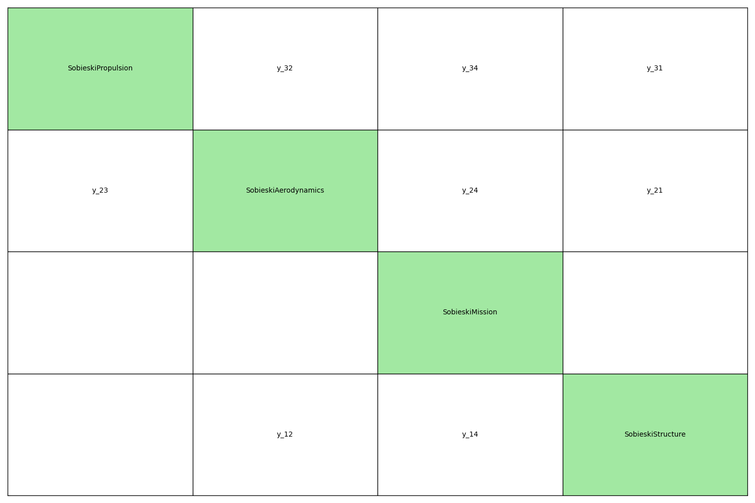
You may also be interested in plotting the couplings of your disciplines.
A quick way of getting this information is the high-level function
generate_n2_plot(). A much more detailed explanation of coupling
visualization is available here.
generate_n2_plot(disciplines, save=False, show=True)
Build, execute and post-process the scenario#
Then, we build the scenario which links the disciplines
with the formulation and the optimization algorithm. Here, we use the
MDF formulation. We tell the scenario to minimize -y_4 instead of
minimizing y_4 (range), which is the default option.
Instantiate the scenario#
During the instantiation of the scenario, we provide some options for the
MDF formulations. The MDF formulation includes an MDA, and thus one of the settings of
the formulation is main_mda_settings, which configures the solver for the strong
couplings.
main_mda_settings = {
    "tolerance": 1e-14,
    "max_mda_iter": 50,
    "warm_start": True,
    "use_lu_fact": False,
    "linear_solver_tolerance": 1e-14,
}
'warm_start: warm starts MDA,'use_lu_fact: optimize the adjoint resolution by storing the Jacobian matrix LU factorization for the multiple RHS (objective + constraints). This saves CPU time if you can pay for the memory and have the full Jacobians available, not just matrix vector products.'linear_solver_tolerance': set the linear solver tolerance, idem we need full convergence
design_space = SobieskiDesignSpace()
design_space
scenario = create_scenario(
    disciplines,
    "y_4",
    design_space,
    maximize_objective=True,
    formulation_name="MDF",
    main_mda_settings=main_mda_settings,
)
Set the design constraints#
for c_name in ["g_1", "g_2", "g_3"]:
    scenario.add_constraint(c_name, constraint_type="ineq")
XDSMIZE the scenario#
Generate the XDSM file on the fly:
log_workflow_status=Truewill log the status of the workflow in the console,save_html(defaultTrue) will generate a self-contained HTML file, that can be automatically opened usingshow_html=True.
scenario.xdsmize(save_html=False)
Define the algorithm inputs#
We set the maximum number of iterations, the optimizer
and the optimizer options. Algorithm specific options are passed there.
Use the high-level function get_algorithm_options_schema()
for more information or read the documentation.
Here the ftol_rel setting is a stop criteria based on the relative difference
in the objective between two iterates ineq_tolerance the tolerance
determination of the optimum; this is specific to the GEMSEO wrapping and not
in the solver.
from gemseo.settings.opt import SLSQP_Settings  # noqa: E402

slsqp_settings = SLSQP_Settings(
    max_iter=10,
    ftol_rel=1e-10,
    ineq_tolerance=2e-3,
    normalize_design_space=True,
)
See also
We can also generate a backup file for the optimization,
as well as plots on the fly of the optimization history if option
plot is True.
This slows down a lot the process, here since SSBJ is very light
scenario.set_optimization_history_backup(
    file_path="mdf_backup.h5",
    at_each_iteration=True,
    at_each_function_call=False,
    erase=True,
    load=False,
    plot=True
)
Execute the scenario#
scenario.execute(slsqp_settings)
   INFO - 16:13:48: *** Start MDOScenario execution ***
   INFO - 16:13:48: MDOScenario
   INFO - 16:13:48:    Disciplines: SobieskiAerodynamics SobieskiMission SobieskiPropulsion SobieskiStructure
   INFO - 16:13:48:    MDO formulation: MDF
   INFO - 16:13:48: Optimization problem:
   INFO - 16:13:48:    minimize -y_4(x_shared, x_1, x_2, x_3)
   INFO - 16:13:48:    with respect to x_1, x_2, x_3, x_shared
   INFO - 16:13:48:    under the inequality constraints
   INFO - 16:13:48:       g_1(x_shared, x_1, x_2, x_3) <= 0
   INFO - 16:13:48:       g_2(x_shared, x_1, x_2, x_3) <= 0
   INFO - 16:13:48:       g_3(x_shared, x_1, x_2, x_3) <= 0
   INFO - 16:13:48:    over the design space:
   INFO - 16:13:48:       +-------------+-------------+-------+-------------+-------+
   INFO - 16:13:48:       | Name        | Lower bound | Value | Upper bound | Type  |
   INFO - 16:13:48:       +-------------+-------------+-------+-------------+-------+
   INFO - 16:13:48:       | x_shared[0] |     0.01    |  0.05 |     0.09    | float |
   INFO - 16:13:48:       | x_shared[1] |    30000    | 45000 |    60000    | float |
   INFO - 16:13:48:       | x_shared[2] |     1.4     |  1.6  |     1.8     | float |
   INFO - 16:13:48:       | x_shared[3] |     2.5     |  5.5  |     8.5     | float |
   INFO - 16:13:48:       | x_shared[4] |      40     |   55  |      70     | float |
   INFO - 16:13:48:       | x_shared[5] |     500     |  1000 |     1500    | float |
   INFO - 16:13:48:       | x_1[0]      |     0.1     |  0.25 |     0.4     | float |
   INFO - 16:13:48:       | x_1[1]      |     0.75    |   1   |     1.25    | float |
   INFO - 16:13:48:       | x_2         |     0.75    |   1   |     1.25    | float |
   INFO - 16:13:48:       | x_3         |     0.1     |  0.5  |      1      | float |
   INFO - 16:13:48:       +-------------+-------------+-------+-------------+-------+
   INFO - 16:13:48: Solving optimization problem with algorithm SLSQP:
   INFO - 16:13:48:     10%|█         | 1/10 [00:00<00:00, 22.28 it/sec, feas=False, obj=-536]
   INFO - 16:13:48:     20%|██        | 2/10 [00:00<00:00, 25.38 it/sec, feas=False, obj=-2.12e+3]
   INFO - 16:13:48:     30%|███       | 3/10 [00:00<00:00, 23.81 it/sec, feas=True, obj=-3.72e+3]
   INFO - 16:13:48:     40%|████      | 4/10 [00:00<00:00, 25.82 it/sec, feas=True, obj=-3.96e+3]
WARNING - 16:13:48: MDAJacobi has reached its maximum number of unsuccessful iterations, but the normalized residual norm 5.126876767779417e-11 is still above the tolerance 1e-14.
   INFO - 16:13:48:     50%|█████     | 5/10 [00:00<00:00, 26.83 it/sec, feas=True, obj=-3.96e+3]
   INFO - 16:13:48: Optimization result:
   INFO - 16:13:48:    Optimizer info:
   INFO - 16:13:48:       Status: 8
   INFO - 16:13:48:       Message: Positive directional derivative for linesearch
   INFO - 16:13:48:    Solution:
   INFO - 16:13:48:       The solution is feasible.
   INFO - 16:13:48:       Objective: -3963.8622159757956
   INFO - 16:13:48:       Standardized constraints:
   INFO - 16:13:48:          g_1 = [-0.01805379 -0.0333412  -0.04424541 -0.05183129 -0.05732327 -0.13720865
   INFO - 16:13:48:  -0.10279135]
   INFO - 16:13:48:          g_2 = 9.423096252181296e-07
   INFO - 16:13:48:          g_3 = [-0.76777633 -0.23222367  0.00080718 -0.183255  ]
   INFO - 16:13:48:       Design space:
   INFO - 16:13:48:          +-------------+-------------+---------------------+-------------+-------+
   INFO - 16:13:48:          | Name        | Lower bound |        Value        | Upper bound | Type  |
   INFO - 16:13:48:          +-------------+-------------+---------------------+-------------+-------+
   INFO - 16:13:48:          | x_shared[0] |     0.01    | 0.06000023557740629 |     0.09    | float |
   INFO - 16:13:48:          | x_shared[1] |    30000    |        60000        |    60000    | float |
   INFO - 16:13:48:          | x_shared[2] |     1.4     |         1.4         |     1.8     | float |
   INFO - 16:13:48:          | x_shared[3] |     2.5     |         2.5         |     8.5     | float |
   INFO - 16:13:48:          | x_shared[4] |      40     |          70         |      70     | float |
   INFO - 16:13:48:          | x_shared[5] |     500     |         1500        |     1500    | float |
   INFO - 16:13:48:          | x_1[0]      |     0.1     |         0.4         |     0.4     | float |
   INFO - 16:13:48:          | x_1[1]      |     0.75    |         0.75        |     1.25    | float |
   INFO - 16:13:48:          | x_2         |     0.75    |         0.75        |     1.25    | float |
   INFO - 16:13:48:          | x_3         |     0.1     |  0.1563708636523273 |      1      | float |
   INFO - 16:13:48:          +-------------+-------------+---------------------+-------------+-------+
   INFO - 16:13:48: *** End MDOScenario execution ***
Save the optimization history#
We can save the whole optimization problem and its history for further post-processing:
scenario.save_optimization_history("mdf_history.h5", file_format="hdf5")
INFO - 16:13:48: Exporting the optimization problem to the file mdf_history.h5
We can also save only calls to functions and design variables history:
scenario.save_optimization_history("mdf_history.xml", file_format="ggobi")
Print optimization metrics#
scenario.print_execution_metrics()
INFO - 16:13:48: The discipline counters are disabled.
Post-process the results#
Plot the optimization history view#
scenario.post_process(post_name="OptHistoryView", save=False, show=True)
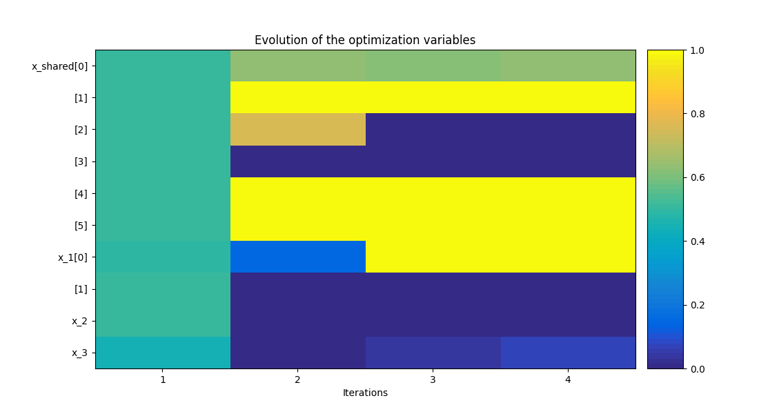
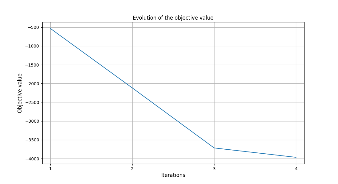
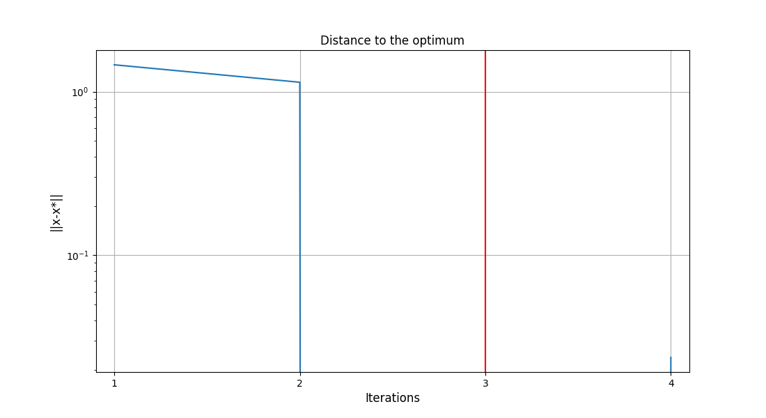
<gemseo.post.opt_history_view.OptHistoryView object at 0x7c4bce44df70>
Note that post-processor settings passed to BaseScenario.post_process can be
provided via a Pydantic model (see the example below). For more information,
see Post-processor Settings.
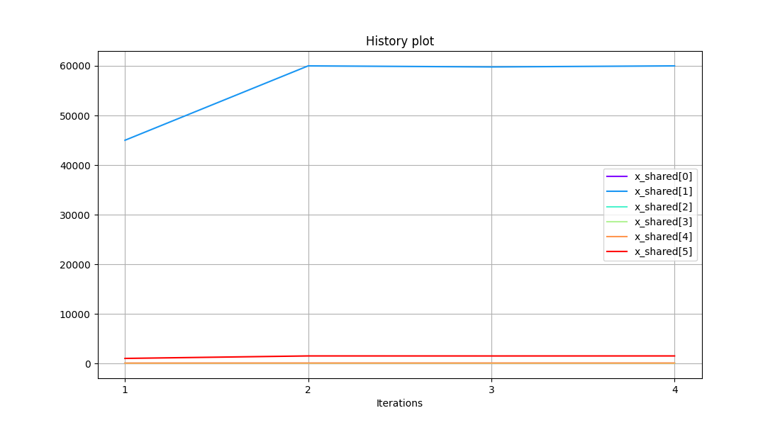
Plot the basic history view#
from gemseo.settings.post import BasicHistory_Settings  # noqa: E402

scenario.post_process(
    BasicHistory_Settings(variable_names=["x_shared"], save=False, show=True)
)
<gemseo.post.basic_history.BasicHistory object at 0x7c4bce44d010>
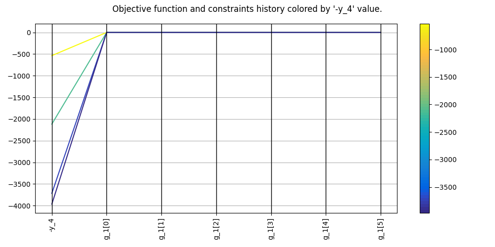
Plot the constraints and objective history#
scenario.post_process(post_name="ObjConstrHist", save=False, show=True)
<gemseo.post.obj_constr_hist.ObjConstrHist object at 0x7c4bce44df70>
Plot the constraints history#
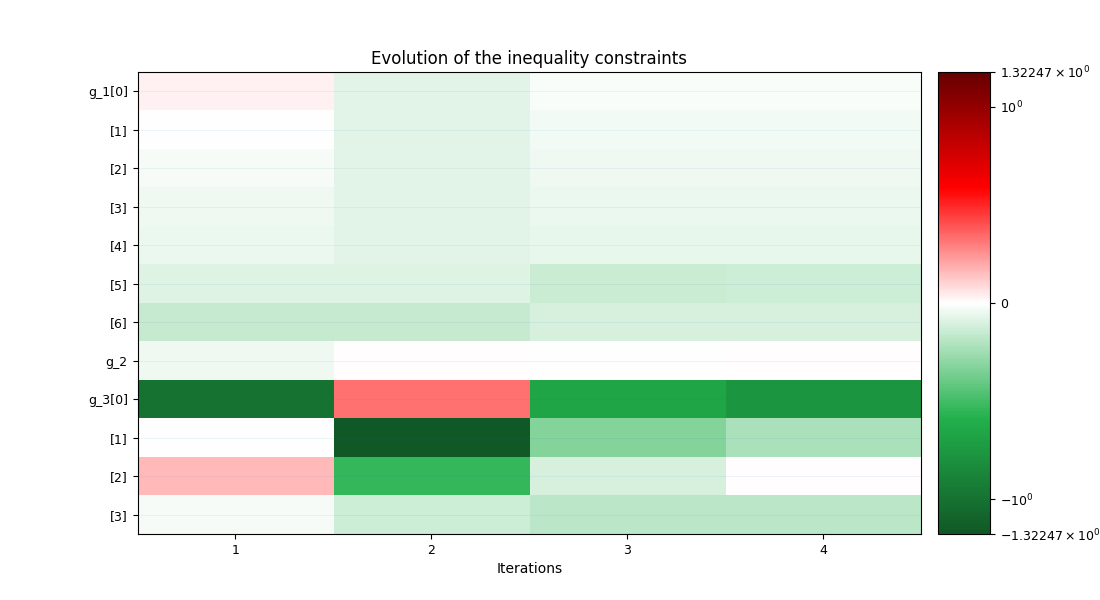
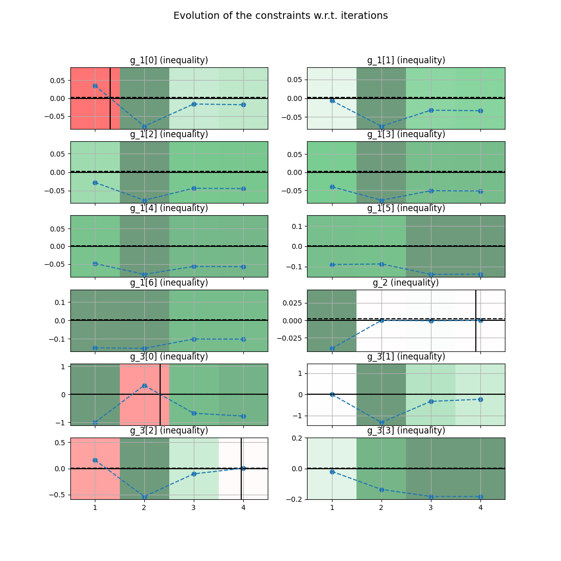
scenario.post_process(
    post_name="ConstraintsHistory",
    constraint_names=["g_1", "g_2", "g_3"],
    save=False,
    show=True,
)
![Evolution of the constraints w.r.t. iterations, g_1[0] (inequality), g_1[1] (inequality), g_1[2] (inequality), g_1[3] (inequality), g_1[4] (inequality), g_1[5] (inequality), g_1[6] (inequality), g_2 (inequality), g_3[0] (inequality), g_3[1] (inequality), g_3[2] (inequality), g_3[3] (inequality)](../../_images/sphx_glr_plot_sobieski_mdf_example_008.png)
<gemseo.post.constraints_history.ConstraintsHistory object at 0x7c4bce536a20>
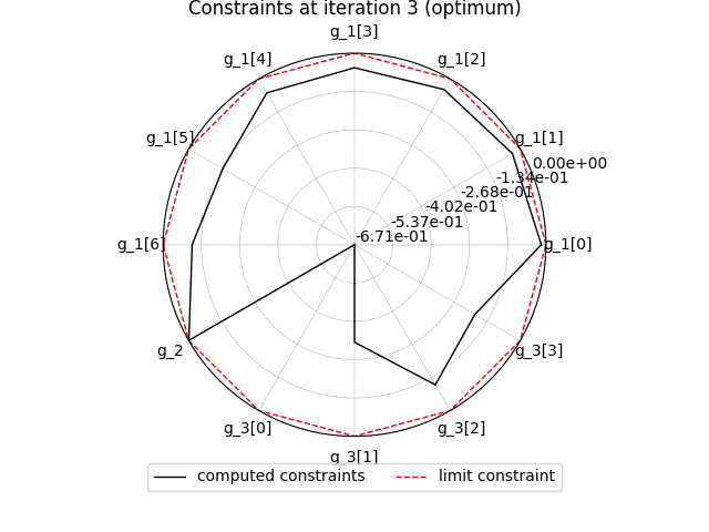
Plot the constraints history using a radar chart#
scenario.post_process(
    post_name="RadarChart",
    constraint_names=["g_1", "g_2", "g_3"],
    save=False,
    show=True,
)
<gemseo.post.radar_chart.RadarChart object at 0x7c4bb2ee4560>
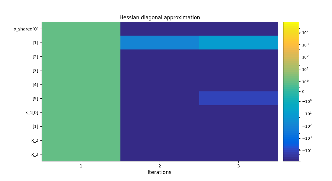
Plot the quadratic approximation of the objective#
scenario.post_process(post_name="QuadApprox", function="-y_4", save=False, show=True)
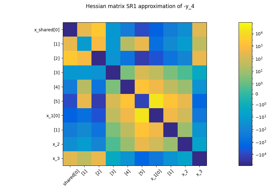
<gemseo.post.quad_approx.QuadApprox object at 0x7c4bbd1bdca0>
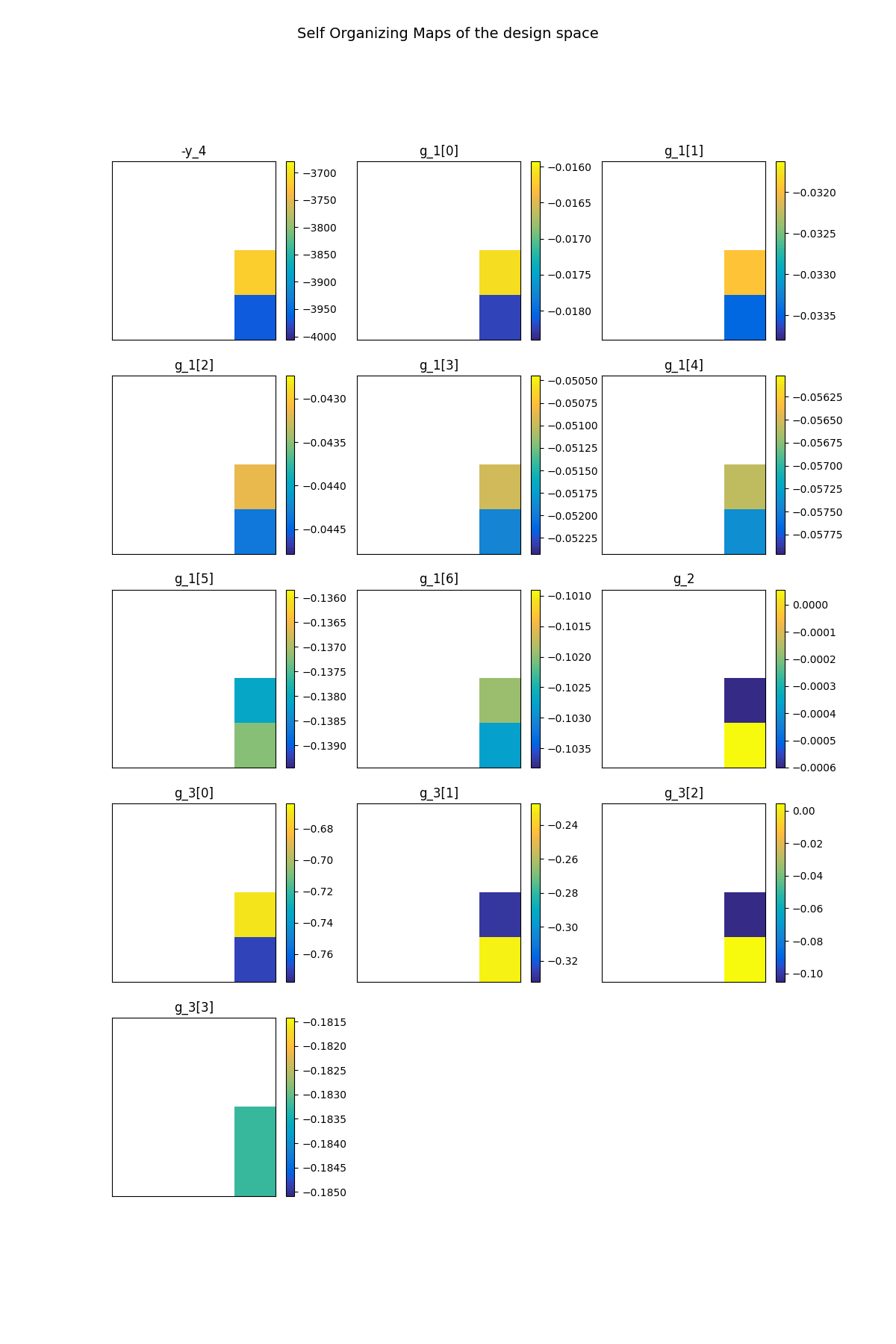
Plot the functions using a SOM#
scenario.post_process(post_name="SOM", save=False, show=True)
![Self Organizing Maps of the design space, -y_4, g_1[0], g_1[1], g_1[2], g_1[3], g_1[4], g_1[5], g_1[6], g_2, g_3[0], g_3[1], g_3[2], g_3[3]](../../_images/sphx_glr_plot_sobieski_mdf_example_012.png)
    INFO - 16:13:50: Building Self Organizing Map from optimization history:
    INFO - 16:13:50:     Number of neurons in x direction = 4
    INFO - 16:13:50:     Number of neurons in y direction = 4

<gemseo.post.som.SOM object at 0x7c4bb32a1eb0>
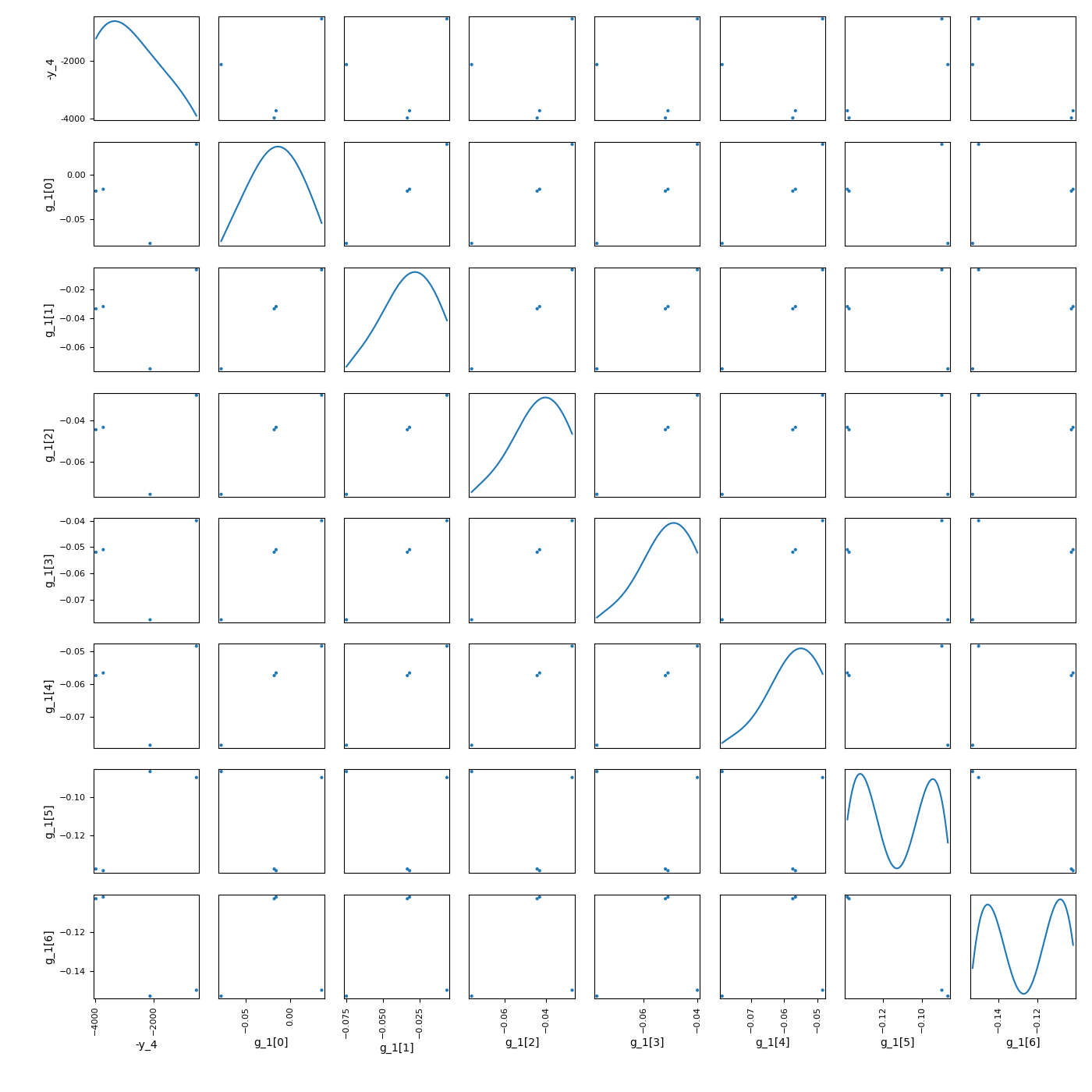
Plot the scatter matrix of variables of interest#
scenario.post_process(
    post_name="ScatterPlotMatrix",
    variable_names=["-y_4", "g_1"],
    save=False,
    show=True,
    fig_size=(14, 14),
)
<gemseo.post.scatter_plot_matrix.ScatterPlotMatrix object at 0x7c4bcf192f90>
Plot the variables using the parallel coordinates#
scenario.post_process(post_name="ParallelCoordinates", save=False, show=True)
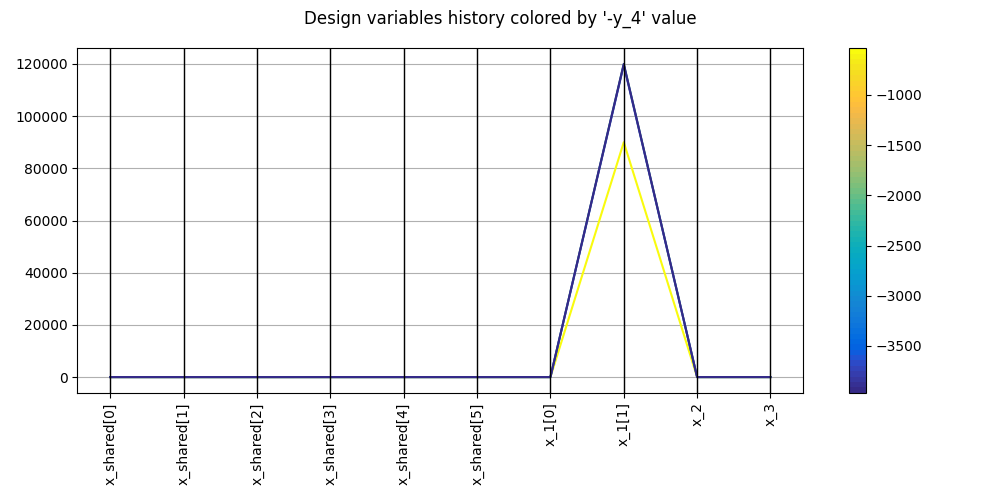
<gemseo.post.parallel_coordinates.ParallelCoordinates object at 0x7c4bb2e8c560>
Plot the robustness of the solution#
scenario.post_process(post_name="Robustness", save=False, show=True)
<gemseo.post.robustness.Robustness object at 0x7c4bcf192f90>
Plot the influence of the design variables#
scenario.post_process(
    post_name="VariableInfluence", fig_size=(14, 14), save=False, show=True
)
![9 variables explain 99% of -y_4, 5 variables explain 99% of g_1[0], 5 variables explain 99% of g_1[1], 5 variables explain 99% of g_1[2], 5 variables explain 99% of g_1[3], 5 variables explain 99% of g_1[4], 4 variables explain 99% of g_1[5], 4 variables explain 99% of g_1[6], 1 variables explain 99% of g_2, 7 variables explain 99% of g_3[0], 7 variables explain 99% of g_3[1], 3 variables explain 99% of g_3[2], 3 variables explain 99% of g_3[3]](../../_images/sphx_glr_plot_sobieski_mdf_example_017.png)
    INFO - 16:13:53: Output name; most influential variables to explain 0.99% of the output variation
    INFO - 16:13:53:    -y_4; x_1[1], x_2, x_3, x_shared[0], x_shared[1], x_shared[2], x_shared[3], x_shared[4], x_shared[5]
    INFO - 16:13:53:    g_1[0]; x_1[0], x_1[1], x_shared[0], x_shared[3], x_shared[5]
    INFO - 16:13:53:    g_1[1]; x_1[0], x_1[1], x_shared[0], x_shared[3], x_shared[5]
    INFO - 16:13:53:    g_1[2]; x_1[0], x_1[1], x_shared[0], x_shared[3], x_shared[5]
    INFO - 16:13:53:    g_1[3]; x_1[0], x_1[1], x_shared[0], x_shared[3], x_shared[5]
    INFO - 16:13:53:    g_1[4]; x_1[0], x_1[1], x_shared[0], x_shared[3], x_shared[5]
    INFO - 16:13:53:    g_1[5]; x_1[0], x_1[1], x_shared[3], x_shared[5]
    INFO - 16:13:53:    g_1[6]; x_1[0], x_1[1], x_shared[3], x_shared[5]
    INFO - 16:13:53:    g_2; x_shared[0]
    INFO - 16:13:53:    g_3[0]; x_2, x_3, x_shared[0], x_shared[1], x_shared[2], x_shared[4], x_shared[5]
    INFO - 16:13:53:    g_3[1]; x_2, x_3, x_shared[0], x_shared[1], x_shared[2], x_shared[4], x_shared[5]
    INFO - 16:13:54:    g_3[2]; x_3, x_shared[1], x_shared[2]
    INFO - 16:13:54:    g_3[3]; x_3, x_shared[1], x_shared[2]

<gemseo.post.variable_influence.VariableInfluence object at 0x7c4bb5fd0380>
Total running time of the script: (0 minutes 5.992 seconds)