Solve an ODE: the Van der Pol problem

from __future__ import annotations

from typing import TYPE_CHECKING

import matplotlib.pyplot as plt
from numpy import array
from numpy import zeros

from gemseo.algos.ode.factory import ODESolverLibraryFactory
from gemseo.algos.ode.ode_problem import ODEProblem
from gemseo.problems.ode.van_der_pol import VanDerPol

if TYPE_CHECKING:
    from gemseo.typing import NumberArray

This tutorial describes how to solve an ordinary differential equation (ODE) problem with GEMSEO. A first-order ODE is a differential equation that can be written as

\[\frac{ds(t)}{dt} = f(t, s(t))\]

where the right-hand side of the equation \(f(t, s(t))\) is a function of time \(t\) and of a state \(s(t)\) that returns another state \(\frac{ds(t)}{dt}\) (see Hartman, Philip (2002) [1964], Ordinary differential equations, Classics in Applied Mathematics, vol. 38, Philadelphia: Society for Industrial and Applied Mathematics). To solve this equation, initial conditions must be set:

\[s(t_0) = s_0\]

For this example, we consider the Van der Pol equation as an example of a time-independent problem.

Solving the Van der Pol time-independent problem

The Van der Pol problem describes the position over time of an oscillator with non-linear damping:

\[\frac{d^2 x(t)}{dt^2} - \mu (1-x^2(t)) \frac{dx(t)}{dt} + x(t) = 0\]

where \(x(t)\) is the position coordinate at time \(t\), and \(\mu\) is the stiffness parameter.

To solve the Van der Pol problem with GEMSEO, we first need to model this second-order equation as a first-order equation. Let \(y = \frac{dx}{dt}\) and \(s = \begin{pmatrix}x\\y\end{pmatrix}\). Then the Van der Pol problem can be rewritten:

\[\begin{split}\frac{ds(t)}{dt} = f(t, s(t)) = \begin{pmatrix} y(t) \\ \mu (1-x^2(t)) y(t) - x(t) \end{pmatrix}\end{split}\]

Step 1 : Defining the problem

mu = 5


def evaluate_f(time: float, state: NumberArray):
    """Evaluate the right-hand side function :math:`f` of the equation.

    Args:
        time: Time at which :math:`f` should be evaluated.
        state: State for which the :math:`f` should be evaluated.

    Returns:
        The value of :math:`f` at `time` and `state`.
    """
    return state[1], mu * state[1] * (1 - state[0] ** 2) - state[0]


initial_state = array([2, -2 / 3])
initial_time = 0.0
final_time = 50.0
ode_problem = ODEProblem(evaluate_f, initial_state, (initial_time, final_time))

By default, the Jacobian of the problem is approximated using the finite difference method. However, it is possible to define an explicit expression of the Jacobian and pass it to the problem. In the case of the Van der Pol problem, this would be:

def evaluate_jac(time: float, state: NumberArray):
    """Evaluate the Jacobian of the function :math:`f`.

    Args:
        time: Time at which the Jacobian should be evaluated.
        state: State for which the Jacobian should be evaluated.

    Returns:
        The value of the Jacobian at `time` and `state`.
    """
    jac = zeros((2, 2))
    jac[1, 0] = -mu * 2 * state[1] * state[0] - 1
    jac[0, 1] = 1
    jac[1, 1] = mu * (1 - state[0] * state[0])
    return jac


ode_problem_with_jacobian = ODEProblem(
    evaluate_f, initial_state, (initial_time, final_time), jac_wrt_state=evaluate_jac
)

Step 2: Solving the ODE problem

Whether the Jacobian is specified or not, once the problem is defined, the ODE solver is called on the ODEProblem by using the ODESolversFactory:

ODESolverLibraryFactory().execute(ode_problem, algo_name="RK45")
ODESolverLibraryFactory().execute(ode_problem_with_jacobian, algo_name="RK45")

ODEResult(times=array([ 0., 50.]), state_trajectories=array([[ 2.        ,  1.26847016],
       [-0.66666667, -0.34017088]]), n_func_evaluations=1730, n_jac_evaluations=0, algorithm_has_converged=True, algorithm_name='RK45', algorithm_settings={'first_step': None, 'max_step': inf, 'rtol': 0.001, 'atol': 1e-06, 't_eval': array([ 0., 50.])}, algorithm_termination_message='The solver successfully reached the end of the integration interval.', terminal_event_index=None, terminal_event_state=array([[ 1.26847016],
       [-0.34017088]]), terminal_event_time=array([50.]))

By default, the Runge-Kutta method of order 4(5) ("RK45") is used, but other algorithms can be applied by specifying the option algo_name in ODESolverLibraryFactory().execute(). See more information on available algorithms in the SciPy documentation.

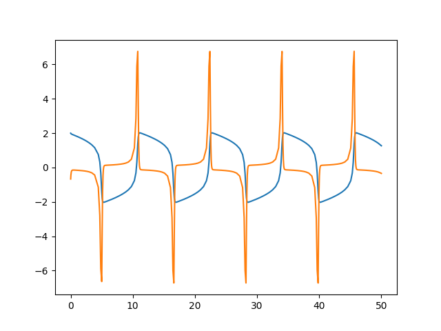
Step 3: Examining the results

The convergence of the algorithm can be known by examining ODEProblem.algorithm_has_converged and ODEProblem.solver_message.

The solution of the ODEProblem on the user-specified time interval can be accessed through the vectors ODEProblem.states and ODEProblem.times.

plt.plot(ode_problem.result.times, ode_problem.result.state_trajectories[0], label="x")
plt.plot(ode_problem.result.times, ode_problem.result.state_trajectories[1], label="y")
plt.legend()
plt.xlabel("time")
plt.show()

Shortcut

The class VanDerPol is available in the package gemseo.problems.ode, so it just needs to be imported to be used.

ode_problem = VanDerPol()
ODESolverLibraryFactory().execute(ode_problem, algo_name="RK45")

ODEResult(times=array([0. , 0.5]), state_trajectories=array([[ 2.00000000e+00,  1.99944457e+00],
       [-6.66543343e-01, -6.67382536e-04]]), n_func_evaluations=3134, n_jac_evaluations=0, algorithm_has_converged=True, algorithm_name='RK45', algorithm_settings={'first_step': None, 'max_step': inf, 'rtol': 0.001, 'atol': 1e-06, 't_eval': array([0. , 0.5])}, algorithm_termination_message='The solver successfully reached the end of the integration interval.', terminal_event_index=None, terminal_event_state=array([[ 1.99944457e+00],
       [-6.67382536e-04]]), terminal_event_time=array([0.5]))