Note
Go to the end to download the full example code.
Store observables#
Introduction#
In this example,
we will learn how to store the history of state variables using the
add_observable() method.
This is useful in situations where we wish to access, post-process,
or save the values of discipline outputs that are not design variables,
constraints or objective functions.
The Sellar problem#
We will consider in this example the Sellar problem:
where the coupling variables are
and
and where the general constraints are
Imports#
All the imports needed for the tutorials are performed here.
from __future__ import annotations

from numpy import array
from numpy import ones

from gemseo import create_discipline
from gemseo import create_scenario
from gemseo.algos.design_space import DesignSpace
Create the problem disciplines#
In this section,
we use the available classes Sellar1, Sellar2
and SellarSystem to define the disciplines of the problem.
The create_discipline() API function allows us to
carry out this task easily, as well as store the instances in a list
to be used later on.
disciplines = create_discipline(["Sellar1", "Sellar2", "SellarSystem"])
Create and execute the scenario#
Create the design space#
In this section, we define the design space which will be used for the creation of the MDOScenario.
design_space = DesignSpace()
design_space.add_variable("x_local", lower_bound=0.0, upper_bound=10.0, value=ones(1))
design_space.add_variable(
    "x_shared",
    2,
    lower_bound=(-10, 0.0),
    upper_bound=(10.0, 10.0),
    value=array([4.0, 3.0]),
)
Create the scenario#
In this section, we build the MDO scenario which links the disciplines with the formulation, the design space and the objective function.
scenario = create_scenario(disciplines, "obj", design_space, formulation_name="MDF")
INFO - 16:12:44: Variable x_local was removed from the Design Space, it is not an input of any discipline.
Note that the formulation settings passed to create_scenario() can be provided
via a Pydantic model. For more information, see Formulation Settings.
Add the constraints#
Then, we have to set the design constraints
scenario.add_constraint("c_1", constraint_type="ineq")
scenario.add_constraint("c_2", constraint_type="ineq")
Add the observables#
Only the design variables, objective function and constraints are stored by
default. In order to be able to recover the data from the state variables,
y1 and y2, we have to add them as observables. All we have to do is enter
the variable name as a string to the
add_observable() method.
If more than one output name is provided (as a list of strings),
the observable function returns a concatenated array of the output values.
scenario.add_observable("y_1")
It is also possible to add the observable with a custom name, using the option observable_name. Let us store the variable y_2 as y2.
scenario.add_observable("y_2", observable_name="y2")
Execute the scenario#
Then, we execute the MDO scenario with the inputs of the MDO scenario as a dictionary. In this example, the gradient-based SLSQP optimizer is selected, with 10 iterations at maximum:
scenario.execute(algo_name="SLSQP", max_iter=10)
INFO - 16:12:44: *** Start MDOScenario execution ***
INFO - 16:12:44: MDOScenario
INFO - 16:12:44:    Disciplines: Sellar1 Sellar2 SellarSystem
INFO - 16:12:44:    MDO formulation: MDF
INFO - 16:12:44: Optimization problem:
INFO - 16:12:44:    minimize obj(x_shared)
INFO - 16:12:44:    with respect to x_shared
INFO - 16:12:44:    under the inequality constraints
INFO - 16:12:44:       c_1(x_shared) <= 0
INFO - 16:12:44:       c_2(x_shared) <= 0
INFO - 16:12:44:    over the design space:
INFO - 16:12:44:       +-------------+-------------+-------+-------------+-------+
INFO - 16:12:44:       | Name        | Lower bound | Value | Upper bound | Type  |
INFO - 16:12:44:       +-------------+-------------+-------+-------------+-------+
INFO - 16:12:44:       | x_shared[0] |     -10     |   4   |      10     | float |
INFO - 16:12:44:       | x_shared[1] |      0      |   3   |      10     | float |
INFO - 16:12:44:       +-------------+-------------+-------+-------------+-------+
INFO - 16:12:44: Solving optimization problem with algorithm SLSQP:
INFO - 16:12:44:     10%|█         | 1/10 [00:00<00:00, 55.17 it/sec, feas=True, obj=19.8]
INFO - 16:12:44:     20%|██        | 2/10 [00:00<00:00, 72.71 it/sec, feas=True, obj=5.38]
INFO - 16:12:44:     30%|███       | 3/10 [00:00<00:00, 82.34 it/sec, feas=True, obj=3.41]
INFO - 16:12:44:     40%|████      | 4/10 [00:00<00:00, 87.54 it/sec, feas=True, obj=3.19]
INFO - 16:12:44:     50%|█████     | 5/10 [00:00<00:00, 91.30 it/sec, feas=True, obj=3.18]
INFO - 16:12:44:     60%|██████    | 6/10 [00:00<00:00, 94.12 it/sec, feas=True, obj=3.18]
INFO - 16:12:44:     70%|███████   | 7/10 [00:00<00:00, 103.02 it/sec, feas=True, obj=3.18]
INFO - 16:12:44:     80%|████████  | 8/10 [00:00<00:00, 110.88 it/sec, feas=True, obj=3.18]
INFO - 16:12:44: Optimization result:
INFO - 16:12:44:    Optimizer info:
INFO - 16:12:44:       Status: None
INFO - 16:12:44:       Message: Successive iterates of the objective function are closer than ftol_rel or ftol_abs. GEMSEO stopped the driver.
INFO - 16:12:44:    Solution:
INFO - 16:12:44:       The solution is feasible.
INFO - 16:12:44:       Objective: 3.183393960638473
INFO - 16:12:44:       Standardized constraints:
INFO - 16:12:44:          c_1 = 1.5724075375089797e-09
INFO - 16:12:44:          c_2 = -20.244722684911245
INFO - 16:12:44:       Design space:
INFO - 16:12:44:          +-------------+-------------+-------------------+-------------+-------+
INFO - 16:12:44:          | Name        | Lower bound |       Value       | Upper bound | Type  |
INFO - 16:12:44:          +-------------+-------------+-------------------+-------------+-------+
INFO - 16:12:44:          | x_shared[0] |     -10     | 1.977638860218251 |      10     | float |
INFO - 16:12:44:          | x_shared[1] |      0      |         0         |      10     | float |
INFO - 16:12:44:          +-------------+-------------+-------------------+-------------+-------+
INFO - 16:12:44: *** End MDOScenario execution (time: 0:00:00.075537) ***
Note that the algorithm settings passed to DriverLibrary.execute() can be provided
via a Pydantic model. For more information, see Algorithm Settings.
Access the observable variables#
Retrieve observables from a dataset#
In order to create a dataset, we use the
corresponding OptimizationProblem:
opt_problem = scenario.formulation.optimization_problem
We can easily build an OptimizationDataset from this OptimizationProblem:
either by separating the design parameters from the functions
(default option):
dataset = opt_problem.to_dataset("sellar_problem")
dataset
or by considering all features as default parameters:
dataset = opt_problem.to_dataset("sellar_problem", categorize=False)
dataset
or by using an input-output naming rather than an optimization naming:
dataset = opt_problem.to_dataset("sellar_problem", opt_naming=False)
dataset
Access observables by name#
We can get the observable data by variable names:
dataset.get_view(variable_names=["y_1", "y2"])
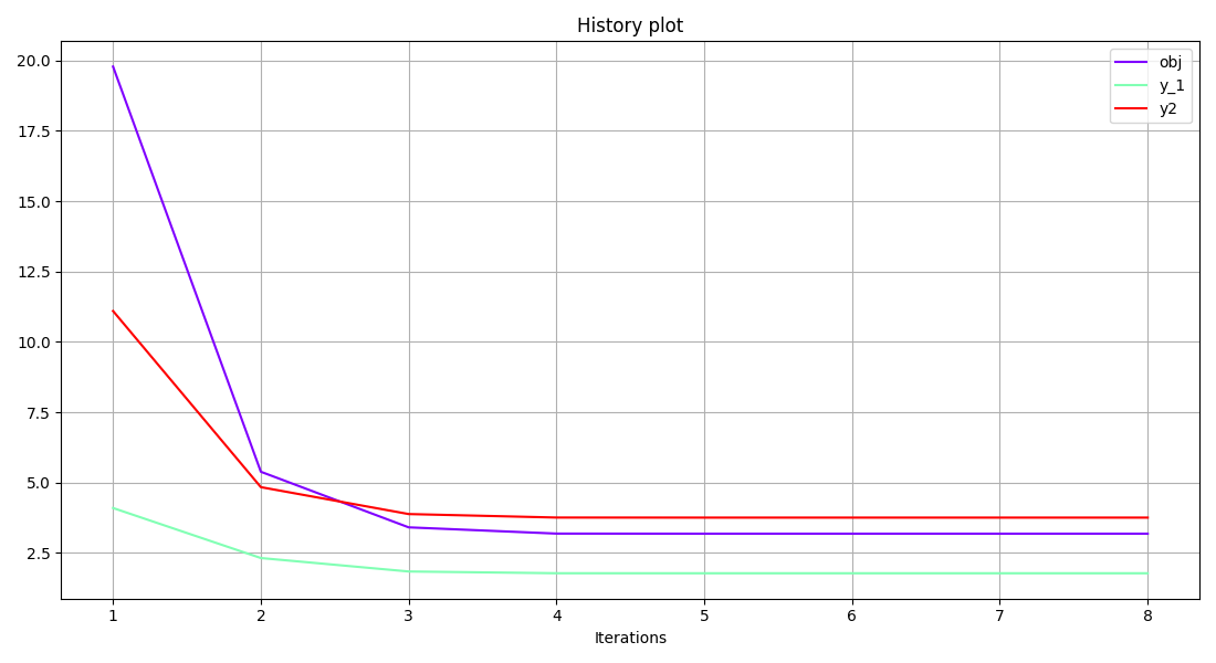
Use the observables in a post-processing method#
Finally, we can generate plots with the observable variables. Have a look at the Basic History plot and the Scatter Plot Matrix:
scenario.post_process(
    post_name="BasicHistory",
    variable_names=["obj", "y_1", "y2"],
    save=False,
    show=True,
)
<gemseo.post.basic_history.BasicHistory object at 0x7c4bbcbf3a40>
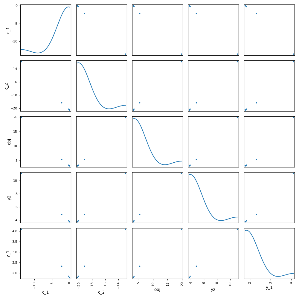
Note that the post-processor settings passed to BaseScenario.post_process() can be
provided via a Pydantic model. For more information, see
Post-processor Settings. An example is shown below.
from gemseo.settings.post import ScatterPlotMatrix_Settings  # noqa: E402

scenario.post_process(
    ScatterPlotMatrix_Settings(
        variable_names=["obj", "c_1", "c_2", "y2", "y_1"],
        save=False,
        show=True,
    )
)
<gemseo.post.scatter_plot_matrix.ScatterPlotMatrix object at 0x7c4bbcbf0200>
Total running time of the script: (0 minutes 0.733 seconds)