Parametric estimation of statistics

In this example, we want to estimate statistics from synthetic data. These data are 500 realizations of x_0, x_1, x_2 and x_3 distributed in the following way:

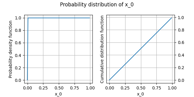
• x_0: standard uniform distribution,

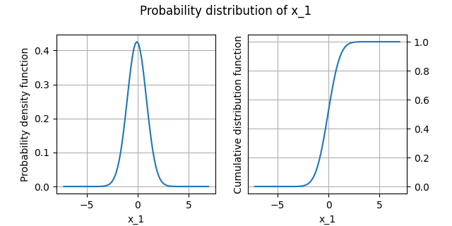
• x_1: standard normal distribution,

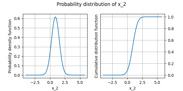
• x_2: standard Weibull distribution,

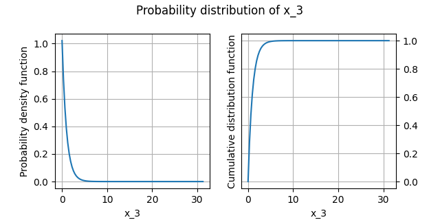
• x_3: standard exponential distribution.

These samples are generated from the NumPy library.

from __future__ import annotations

from numpy import vstack
from numpy.random import default_rng

from gemseo import configure_logger
from gemseo import create_dataset
from gemseo.uncertainty import create_statistics

configure_logger()

<RootLogger root (INFO)>

Create synthetic data

rng = default_rng(0)

n_samples = 500

uniform_rand = rng.uniform(size=n_samples)
normal_rand = rng.normal(size=n_samples)
weibull_rand = rng.weibull(1.5, size=n_samples)
exponential_rand = rng.exponential(size=n_samples)

data = vstack((uniform_rand, normal_rand, weibull_rand, exponential_rand)).T

variables = ["x_0", "x_1", "x_2", "x_3"]

data

array([[ 6.36961687e-01,  1.35543803e+00,  1.24477385e-01,
         1.91363961e-01],
       [ 2.69786714e-01,  2.21160257e-03,  8.14109465e-01,
         2.33137384e+00],
       [ 4.09735239e-02, -7.90544810e-01,  4.64297251e-01,
         5.53852517e-01],
       ...,
       [ 9.85769635e-01, -1.16187331e+00,  9.62671893e-01,
         8.66423178e-01],
       [ 4.28024519e-01,  2.72032137e-01,  5.03249648e-01,
         2.17492296e-01],
       [ 8.43014715e-01, -7.66939588e-01,  8.18740909e-01,
         8.75593057e-01]])

Create a ParametricStatistics object

We create a ParametricStatistics object from this data encapsulated in a Dataset:

dataset = create_dataset("Dataset", data, variables)

and a list of names of candidate probability distributions: exponential, normal and uniform distributions (see ParametricStatistics.DistributionName). We do not use the default fitting criterion (‘BIC’) but ‘Kolmogorov’ (see ParametricStatistics.FittingCriterion and ParametricStatistics.SignificanceTest).

tested_distributions = ["Exponential", "Normal", "Uniform"]
analysis = create_statistics(
    dataset, tested_distributions=tested_distributions, fitting_criterion="Kolmogorov"
)
analysis

   INFO - 13:52:41: Create ParametricStatistics(Dataset), a ParametricStatistics library.
   INFO - 13:52:41: | Set goodness-of-fit criterion: Kolmogorov.
   INFO - 13:52:41: | Set significance level of hypothesis test: 0.05.
   INFO - 13:52:41: Fit different distributions (Exponential, Normal, Uniform) per variable and compute the goodness-of-fit criterion.
   INFO - 13:52:41: | Fit different distributions for x_0.
   INFO - 13:52:41: | Fit different distributions for x_1.
   INFO - 13:52:41: | Fit different distributions for x_2.
   INFO - 13:52:41: | Fit different distributions for x_3.
   INFO - 13:52:41: Select the best distribution for each variable.
WARNING - 13:52:41: All criteria values are lower than the significance level 0.05.
   INFO - 13:52:41: | The best distribution for x_0[0] is Uniform([-0.00168518,0.999196]).
   INFO - 13:52:41: | The best distribution for x_1[0] is Normal([-0.068321,0.937168]).
WARNING - 13:52:41: All criteria values are lower than the significance level 0.05.
   INFO - 13:52:41: | The best distribution for x_2[0] is Normal([0.905464,0.645926]).
   INFO - 13:52:41: | The best distribution for x_3[0] is Exponential([1.02161,0.00146538]).

ParametricStatistics(Dataset)

• n_samples: 500
• n_variables: 4
• variables: x_0, x_1, x_2, x_3

Print the fitting matrix

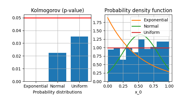
At this step, an optimal distribution has been selected for each variable based on the tested distributions and on the Kolmogorov fitting criterion. We can print the fitting matrix to see the goodness-of-fit measures for each pair < variable, distribution > as well as the selected distribution for each variable. Note that in the case of significance tests, the goodness-of-fit measures are the p-values.

analysis.get_fitting_matrix()

'+----------+------------------------+------------------------+-------------------------+-------------+\n| Variable |      Exponential       |         Normal         |         Uniform         |  Selection  |\n+----------+------------------------+------------------------+-------------------------+-------------+\n|   x_0    | 1.3319194027726772e-16 |  0.02244629355147776   |   0.035215303972709444  |   Uniform   |\n|   x_1    | 1.177360930542324e-55  |   0.9894613754182425   |  2.773038784889384e-21  |    Normal   |\n|   x_2    | 1.624812325803554e-08  | 0.00024649291266878377 |  8.697307474207096e-95  |    Normal   |\n|   x_3    |   0.6841041353514807   | 1.1084730889960638e-13 | 1.0968178545541834e-160 | Exponential |\n+----------+------------------------+------------------------+-------------------------+-------------+'

One can also plot the tested distributions over an histogram of the data as well as the corresponding values of the Kolmogorov fitting criterion:

analysis.plot_criteria("x_0")

<Figure size 640x320 with 2 Axes>

Get statistics

From this ParametricStatistics instance, we can easily get statistics for the different variables based on the selected distributions.

Get minimum

Here is the minimum value for the different variables:

analysis.compute_minimum()

{'x_0': array([-0.00168518]), 'x_1': array([-inf]), 'x_2': array([-inf]), 'x_3': array([0.00146538])}

Get maximum

Here is the minimum value for the different variables:

analysis.compute_maximum()

{'x_0': array([0.99919581]), 'x_1': array([inf]), 'x_2': array([inf]), 'x_3': array([inf])}

Get range

Here is the range, i.e. the difference between the minimum and maximum values, for the different variables:

analysis.compute_range()

{'x_0': array([1.000881]), 'x_1': array([inf]), 'x_2': array([inf]), 'x_3': array([inf])}

Get mean

Here is the mean value for the different variables:

analysis.compute_mean()

{'x_0': array([0.49875531]), 'x_1': array([-0.06832097]), 'x_2': array([0.90546442]), 'x_3': array([0.98031191])}

Get standard deviation

Here is the standard deviation for the different variables:

analysis.compute_standard_deviation()

{'x_0': array([0.28892946]), 'x_1': array([0.93716844]), 'x_2': array([0.64592637]), 'x_3': array([0.97884653])}

Get variance

Here is the variance for the different variables:

analysis.compute_variance()

{'x_0': array([0.08348023]), 'x_1': array([0.87828468]), 'x_2': array([0.41722087]), 'x_3': array([0.95814053])}

Get quantile

Here is the quantile with level 80% for the different variables:

analysis.compute_quantile(0.8)

{'x_0': array([0.79901961]), 'x_1': array([0.72041989]), 'x_2': array([1.44908977]), 'x_3': array([1.5768581])}

Get quartile

Here is the second quartile for the different variables:

analysis.compute_quartile(2)

{'x_0': array([0.49875531]), 'x_1': array([-0.06832097]), 'x_2': array([0.90546442]), 'x_3': array([0.67995009])}

Get percentile

Here is the 50th percentile for the different variables:

analysis.compute_percentile(50)

{'x_0': array([0.49875531]), 'x_1': array([-0.06832097]), 'x_2': array([0.90546442]), 'x_3': array([0.67995009])}

Get median

Here is the median for the different variables:

analysis.compute_median()

{'x_0': array([0.49875531]), 'x_1': array([-0.06832097]), 'x_2': array([0.90546442]), 'x_3': array([0.67995009])}

Get tolerance interval

Here is the two-sided tolerance interval with a coverage level equal to 50% with a confidence level of 95% for the different variables:

analysis.compute_tolerance_interval(0.5)

{'x_0': [Bounds(lower=array([0.24854773]), upper=array([0.75453424]))], 'x_1': [Bounds(lower=array([-0.73596335]), upper=array([0.59932142]))], 'x_2': [Bounds(lower=array([0.44530401]), upper=array([1.36562484]))], 'x_3': [Bounds(lower=array([0.24115604]), upper=array([1.32178328]))]}

Get B-value

Here is the B-value for the different variables, which is a left-sided tolerance interval with a coverage level equal to 90% with a confidence level of 95%:

analysis.compute_b_value()

{'x_0': array([[0.09841318]]), 'x_1': array([[-1.33841706]]), 'x_2': array([[0.0300737]]), 'x_3': array([[0.09423241]])}

Plot the distribution

We can draw the empirical cumulative distribution function and the empirical probability density function:

analysis.plot()

• 
• 
• 
• 

{'x_0': <Figure size 640x320 with 2 Axes>, 'x_1': <Figure size 640x320 with 2 Axes>, 'x_2': <Figure size 640x320 with 2 Axes>, 'x_3': <Figure size 640x320 with 2 Axes>}