Note
Click here to download the full example code
Store observables
- Introduction
In this example, we will learn how to store the history of state variables using the
add_observable()method. This is useful in situations where we wish to access, post-process, or save the values of discipline outputs that are not design variables, constraints or objective functions.
We will consider in this example the Sellar problem:
\[\begin{split}\begin{aligned} \text{minimize the objective function }&obj=x_{local}^2 + x_{shared,2} +y_1^2+e^{-y_2} \\ \text{with respect to the design variables }&x_{shared},\,x_{local} \\ \text{subject to the general constraints } & c_1 \leq 0\\ & c_2 \leq 0\\ \text{subject to the bound constraints } & -10 \leq x_{shared,1} \leq 10\\ & 0 \leq x_{shared,2} \leq 10\\ & 0 \leq x_{local} \leq 10. \end{aligned}\end{split}\]where the coupling variables are
\[\text{Discipline 1: } y_1 = \sqrt{x_{shared,1}^2 + x_{shared,2} + x_{local} - 0.2\,y_2},\]and
\[\text{Discipline 2: }y_2 = |y_1| + x_{shared,1} + x_{shared,2}.\]and where the general constraints are
\[ \begin{align}\begin{aligned}c_1 = 3.16 - y_1^2\\c_2 = y_2 - 24.\end{aligned}\end{align} \]
All the imports needed for the tutorials are performed here.
from gemseo.algos.design_space import DesignSpace
from gemseo.api import configure_logger
from gemseo.api import create_discipline
from gemseo.api import create_scenario
from matplotlib import pyplot as plt
from numpy import array
from numpy import ones

configure_logger()
Out:
<RootLogger root (INFO)>
Create the problem disciplines
In this section,
we use the available classes Sellar1, Sellar2
and SellarSystem to define the disciplines of the problem.
The create_discipline() API function allows us to
carry out this task easily, as well as store the instances in a list
to be used later on.
disciplines = create_discipline(["Sellar1", "Sellar2", "SellarSystem"])
Create and execute the scenario
Create the design space
In this section, we define the design space which will be used for the creation of the MDOScenario.
design_space = DesignSpace()
design_space.add_variable("x_local", 1, l_b=0.0, u_b=10.0, value=ones(1))
design_space.add_variable(
    "x_shared", 2, l_b=(-10, 0.0), u_b=(10.0, 10.0), value=array([4.0, 3.0])
)
Create the scenario
In this section, we build the MDO scenario which links the disciplines with the formulation, the design space and the objective function.
scenario = create_scenario(
    disciplines, formulation="MDF", objective_name="obj", design_space=design_space
)
Add the constraints
Then, we have to set the design constraints
scenario.add_constraint("c_1", "ineq")
scenario.add_constraint("c_2", "ineq")
Add the observables
Only the design variables, objective function and constraints are stored by
default. In order to be able to recover the data from the state variables,
y1 and y2, we have to add them as observables. All we have to do is enter
the variable name as a string to the
add_observable() method.
If more than one output name is provided (as a list of strings),
the observable function returns a concatenated array of the output values.
scenario.add_observable("y_1")
It is also possible to add the observable with a custom name, using the option observable_name. Let us store the variable y_2 as y2.
scenario.add_observable("y_2", observable_name="y2")
Execute the scenario
Then, we execute the MDO scenario with the inputs of the MDO scenario as a dictionary. In this example, the gradient-based SLSQP optimizer is selected, with 10 iterations at maximum:
scenario.execute(input_data={"max_iter": 10, "algo": "SLSQP"})
Out:
    INFO - 07:17:21:
    INFO - 07:17:21: *** Start MDOScenario execution ***
    INFO - 07:17:21: MDOScenario
    INFO - 07:17:21:    Disciplines: Sellar1 Sellar2 SellarSystem
    INFO - 07:17:21:    MDO formulation: MDF
    INFO - 07:17:21: Optimization problem:
    INFO - 07:17:21:    minimize obj(x_local, x_shared)
    INFO - 07:17:21:    with respect to x_local, x_shared
    INFO - 07:17:21:    subject to constraints:
    INFO - 07:17:21:       c_1(x_local, x_shared) <= 0.0
    INFO - 07:17:21:       c_2(x_local, x_shared) <= 0.0
    INFO - 07:17:21:    over the design space:
    INFO - 07:17:21:    +----------+-------------+-------+-------------+-------+
    INFO - 07:17:21:    | name     | lower_bound | value | upper_bound | type  |
    INFO - 07:17:21:    +----------+-------------+-------+-------------+-------+
    INFO - 07:17:21:    | x_local  |      0      |   1   |      10     | float |
    INFO - 07:17:21:    | x_shared |     -10     |   4   |      10     | float |
    INFO - 07:17:21:    | x_shared |      0      |   3   |      10     | float |
    INFO - 07:17:21:    +----------+-------------+-------+-------------+-------+
    INFO - 07:17:21: Solving optimization problem with algorithm SLSQP:
    INFO - 07:17:21: ...   0%|          | 0/10 [00:00<?, ?it]
/home/docs/checkouts/readthedocs.org/user_builds/gemseo/envs/4.0.0/lib/python3.9/site-packages/scipy/optimize/slsqp.py:427: ComplexWarning: Casting complex values to real discards the imaginary part
  slsqp(m, meq, x, xl, xu, fx, c, g, a, acc, majiter, mode, w, jw,
    INFO - 07:17:21: ...  30%|███       | 3/10 [00:00<00:00, 97.89 it/sec, obj=3.41+j]
    INFO - 07:17:21: ...  60%|██████    | 6/10 [00:00<00:00, 47.36 it/sec, obj=3.18+j]
    INFO - 07:17:21: ...  80%|████████  | 8/10 [00:00<00:00, 38.40 it/sec, obj=3.18+j]
    INFO - 07:17:21: Optimization result:
    INFO - 07:17:21:    Optimizer info:
    INFO - 07:17:21:       Status: None
    INFO - 07:17:21:       Message: Successive iterates of the objective function are closer than ftol_rel or ftol_abs. GEMSEO Stopped the driver
    INFO - 07:17:21:       Number of calls to the objective function by the optimizer: 9
    INFO - 07:17:21:    Solution:
    INFO - 07:17:21:       The solution is feasible.
    INFO - 07:17:21:       Objective: (3.1833939452393087+0j)
    INFO - 07:17:21:       Standardized constraints:
    INFO - 07:17:21:          c_1 = (6.486713388653698e-09+0j)
    INFO - 07:17:21:          c_2 = (-20.244722236724627+0j)
    INFO - 07:17:21:       Design space:
    INFO - 07:17:21:       +----------+-------------+-------------------+-------------+-------+
    INFO - 07:17:21:       | name     | lower_bound |       value       | upper_bound | type  |
    INFO - 07:17:21:       +----------+-------------+-------------------+-------------+-------+
    INFO - 07:17:21:       | x_local  |      0      |         0         |      10     | float |
    INFO - 07:17:21:       | x_shared |     -10     | 1.977638881636786 |      10     | float |
    INFO - 07:17:21:       | x_shared |      0      |         0         |      10     | float |
    INFO - 07:17:21:       +----------+-------------+-------------------+-------------+-------+
    INFO - 07:17:21: *** End MDOScenario execution (time: 0:00:00.271076) ***

{'max_iter': 10, 'algo': 'SLSQP'}
Access the observable variables
Retrieve observables from a dataset
In order to create a dataset, we use the
corresponding OptimizationProblem:
opt_problem = scenario.formulation.opt_problem
We can easily build a dataset from this OptimizationProblem:
either by separating the design parameters from the functions
(default option):
dataset = opt_problem.export_to_dataset("sellar_problem")
print(dataset)
Out:
sellar_problem
   Number of samples: 8
   Number of variables: 7
   Variables names and sizes by group:
      design_parameters: x_local (1), x_shared (2)
      functions: c_1 (1), c_2 (1), obj (1), y2 (1), y_1 (1)
   Number of dimensions (total = 8) by group:
      design_parameters: 3
      functions: 5
or by considering all features as default parameters:
dataset = opt_problem.export_to_dataset("sellar_problem", categorize=False)
print(dataset)
Out:
sellar_problem
   Number of samples: 8
   Number of variables: 7
   Variables names and sizes by group:
      parameters: x_local (1), x_shared (2), c_1 (1), c_2 (1), obj (1), y2 (1), y_1 (1)
   Number of dimensions (total = 8) by group:
      parameters: 8
or by using an input-output naming rather than an optimization naming:
dataset = opt_problem.export_to_dataset("sellar_problem", opt_naming=False)
print(dataset)
Out:
sellar_problem
   Number of samples: 8
   Number of variables: 7
   Variables names and sizes by group:
      inputs: x_local (1), x_shared (2)
      outputs: c_1 (1), c_2 (1), obj (1), y2 (1), y_1 (1)
   Number of dimensions (total = 8) by group:
      inputs: 3
      outputs: 5
Access observables by name
We can get the observable data by name, either as a dictionary indexed by the observable names (default option):
print(dataset.get_data_by_names(["y_1", "y2"]))
Out:
{'y_1': array([[4.21393092+0.j],
       [2.32004903+0.j],
       [1.84120131+0.j],
       [1.77871073+0.j],
       [1.77763921+0.j],
       [1.77763888+0.j],
       [1.77763888+0.j],
       [1.77763888+0.j]]), 'y2': array([[11.21393092+0.j],
       [ 4.84009806+0.j],
       [ 3.88161141+0.j],
       [ 3.75742147+0.j],
       [ 3.75527841+0.j],
       [ 3.75527777+0.j],
       [ 3.75527776+0.j],
       [ 3.75527777+0.j]])}
or as an array:
print(dataset.get_data_by_names(["y_1", "y2"], False))
Out:
[[ 4.21393092+0.j 11.21393092+0.j]
 [ 2.32004903+0.j  4.84009806+0.j]
 [ 1.84120131+0.j  3.88161141+0.j]
 [ 1.77871073+0.j  3.75742147+0.j]
 [ 1.77763921+0.j  3.75527841+0.j]
 [ 1.77763888+0.j  3.75527777+0.j]
 [ 1.77763888+0.j  3.75527776+0.j]
 [ 1.77763888+0.j  3.75527777+0.j]]
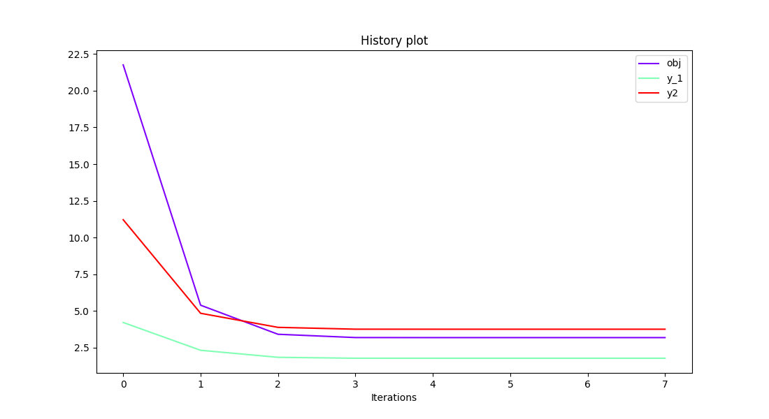
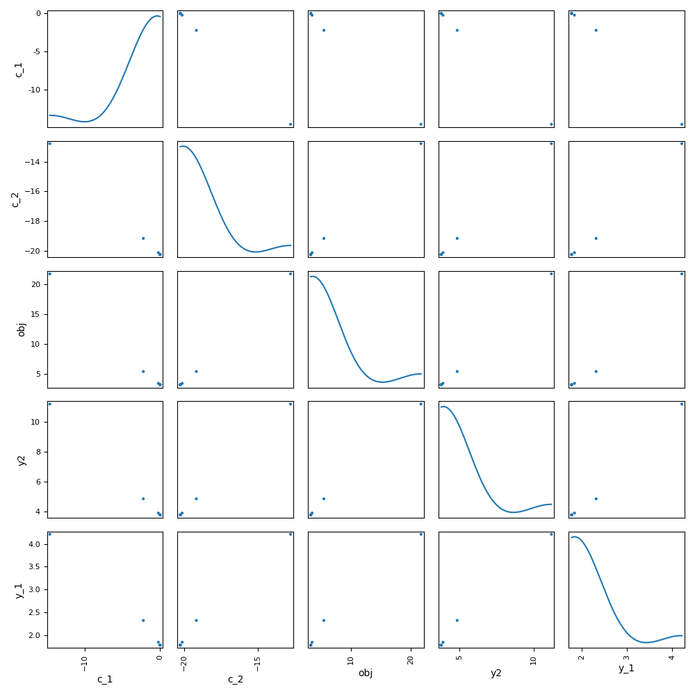
Use the observables in a post-processing method
Finally, we can generate plots with the observable variables. Have a look at the Basic History plot and the Scatter Plot Matrix:
scenario.post_process(
    "BasicHistory", variable_names=["obj", "y_1", "y2"], save=False, show=False
)
scenario.post_process(
    "ScatterPlotMatrix",
    save=False,
    show=False,
    variable_names=["obj", "c_1", "c_2", "y2", "y_1"],
)
# Workaround for HTML rendering, instead of ``show=True``
plt.show()
Out:
/home/docs/checkouts/readthedocs.org/user_builds/gemseo/envs/4.0.0/lib/python3.9/site-packages/matplotlib/cbook/__init__.py:1298: ComplexWarning: Casting complex values to real discards the imaginary part
  return np.asarray(x, float)
/home/docs/checkouts/readthedocs.org/user_builds/gemseo/envs/4.0.0/lib/python3.9/site-packages/gemseo/algos/database.py:1331: VisibleDeprecationWarning: Creating an ndarray from ragged nested sequences (which is a list-or-tuple of lists-or-tuples-or ndarrays with different lengths or shapes) is deprecated. If you meant to do this, you must specify 'dtype=object' when creating the ndarray.
  f_history = array(flat_vals).real
Total running time of the script: ( 0 minutes 1.485 seconds)