Note
Click here to download the full example code
Self-Organizing Map
In this example, we illustrate the use of the SOM plot
on the Sobieski’s SSBJ problem.
from gemseo.api import configure_logger
from gemseo.api import create_discipline
from gemseo.api import create_scenario
from gemseo.problems.sobieski.core.problem import SobieskiProblem
from matplotlib import pyplot as plt
Import
The first step is to import some functions from the API and a method to get the design space.
configure_logger()
Out:
<RootLogger root (INFO)>
Description
The SOM post-processing performs a Self Organizing Map
clustering on the optimization history.
A SOM is a 2D representation of a design of experiments
which requires dimensionality reduction since it may be in a very high dimension.
A SOM is built by using an unsupervised artificial neural network
[KSH01].
A map of size n_x.n_y is generated, where
n_x is the number of neurons in the \(x\) direction and n_y
is the number of neurons in the \(y\) direction. The design space
(whatever the dimension) is reduced to a 2D representation based on
n_x.n_y neurons. Samples are clustered to a neuron when their design
variables are close in terms of their L2 norm. A neuron is always located at the
same place on a map. Each neuron is colored according to the average value for
a given criterion. This helps to qualitatively analyze whether parts of the design
space are good according to some criteria and not for others, and where
compromises should be made. A white neuron has no sample associated with
it: not enough evaluations were provided to train the SOM.
SOM’s provide a qualitative view of the objective function, the constraints, and of their relative behaviors.
Create disciplines
At this point, we instantiate the disciplines of Sobieski’s SSBJ problem: Propulsion, Aerodynamics, Structure and Mission
disciplines = create_discipline(
    [
        "SobieskiPropulsion",
        "SobieskiAerodynamics",
        "SobieskiStructure",
        "SobieskiMission",
    ]
)
Create design space
We also read the design space from the SobieskiProblem.
design_space = SobieskiProblem().design_space
Create and execute scenario
The next step is to build an MDO scenario in order to maximize the range, encoded ‘y_4’, with respect to the design parameters, while satisfying the inequality constraints ‘g_1’, ‘g_2’ and ‘g_3’. We can use the MDF formulation, the Monte Carlo DOE algorithm and 30 samples.
scenario = create_scenario(
    disciplines,
    formulation="MDF",
    objective_name="y_4",
    maximize_objective=True,
    design_space=design_space,
    scenario_type="DOE",
)
scenario.set_differentiation_method("user")
for constraint in ["g_1", "g_2", "g_3"]:
    scenario.add_constraint(constraint, "ineq")
scenario.execute({"algo": "OT_MONTE_CARLO", "n_samples": 30})
Out:
    INFO - 10:03:11:
    INFO - 10:03:11: *** Start DOEScenario execution ***
    INFO - 10:03:11: DOEScenario
    INFO - 10:03:11:    Disciplines: SobieskiPropulsion SobieskiAerodynamics SobieskiStructure SobieskiMission
    INFO - 10:03:11:    MDO formulation: MDF
    INFO - 10:03:11: Optimization problem:
    INFO - 10:03:11:    minimize -y_4(x_shared, x_1, x_2, x_3)
    INFO - 10:03:11:    with respect to x_1, x_2, x_3, x_shared
    INFO - 10:03:11:    subject to constraints:
    INFO - 10:03:11:       g_1(x_shared, x_1, x_2, x_3) <= 0.0
    INFO - 10:03:11:       g_2(x_shared, x_1, x_2, x_3) <= 0.0
    INFO - 10:03:11:       g_3(x_shared, x_1, x_2, x_3) <= 0.0
    INFO - 10:03:11:    over the design space:
    INFO - 10:03:11:    +----------+-------------+-------+-------------+-------+
    INFO - 10:03:11:    | name     | lower_bound | value | upper_bound | type  |
    INFO - 10:03:11:    +----------+-------------+-------+-------------+-------+
    INFO - 10:03:11:    | x_shared |     0.01    |  0.05 |     0.09    | float |
    INFO - 10:03:11:    | x_shared |    30000    | 45000 |    60000    | float |
    INFO - 10:03:11:    | x_shared |     1.4     |  1.6  |     1.8     | float |
    INFO - 10:03:11:    | x_shared |     2.5     |  5.5  |     8.5     | float |
    INFO - 10:03:11:    | x_shared |      40     |   55  |      70     | float |
    INFO - 10:03:11:    | x_shared |     500     |  1000 |     1500    | float |
    INFO - 10:03:11:    | x_1      |     0.1     |  0.25 |     0.4     | float |
    INFO - 10:03:11:    | x_1      |     0.75    |   1   |     1.25    | float |
    INFO - 10:03:11:    | x_2      |     0.75    |   1   |     1.25    | float |
    INFO - 10:03:11:    | x_3      |     0.1     |  0.5  |      1      | float |
    INFO - 10:03:11:    +----------+-------------+-------+-------------+-------+
    INFO - 10:03:11: Solving optimization problem with algorithm OT_MONTE_CARLO:
    INFO - 10:03:11: Generation of OT_MONTE_CARLO DOE with OpenTURNS
    INFO - 10:03:11: ...   0%|          | 0/30 [00:00<?, ?it]
    INFO - 10:03:11: ...   3%|▎         | 1/30 [00:00<00:00, 273.45 it/sec]
    INFO - 10:03:11: ...  13%|█▎        | 4/30 [00:00<00:00, 125.55 it/sec]
    INFO - 10:03:11: ...  23%|██▎       | 7/30 [00:00<00:00, 81.68 it/sec]
    INFO - 10:03:12: ...  33%|███▎      | 10/30 [00:00<00:00, 58.15 it/sec]
    INFO - 10:03:12: ...  43%|████▎     | 13/30 [00:00<00:00, 42.80 it/sec]
    INFO - 10:03:12: ...  50%|█████     | 15/30 [00:00<00:00, 36.32 it/sec]
    INFO - 10:03:12: ...  57%|█████▋    | 17/30 [00:00<00:00, 32.07 it/sec]
    INFO - 10:03:12: ...  63%|██████▎   | 19/30 [00:01<00:00, 28.45 it/sec]
    INFO - 10:03:12: ...  73%|███████▎  | 22/30 [00:01<00:00, 25.09 it/sec]
    INFO - 10:03:12: ...  80%|████████  | 24/30 [00:01<00:00, 22.87 it/sec]
    INFO - 10:03:13: ...  90%|█████████ | 27/30 [00:01<00:00, 20.48 it/sec]
    INFO - 10:03:13: ... 100%|██████████| 30/30 [00:01<00:00, 18.83 it/sec]
    INFO - 10:03:13: ... 100%|██████████| 30/30 [00:01<00:00, 18.80 it/sec]
    INFO - 10:03:13: Optimization result:
    INFO - 10:03:13:    Optimizer info:
    INFO - 10:03:13:       Status: None
    INFO - 10:03:13:       Message: None
    INFO - 10:03:13:       Number of calls to the objective function by the optimizer: 30
    INFO - 10:03:13:    Solution:
    INFO - 10:03:13:       The solution is feasible.
    INFO - 10:03:13:       Objective: -367.45739115001027
    INFO - 10:03:13:       Standardized constraints:
    INFO - 10:03:13:          g_1 = [-0.02478574 -0.00310924 -0.00855146 -0.01702654 -0.02484732 -0.04764585
    INFO - 10:03:13:  -0.19235415]
    INFO - 10:03:13:          g_2 = -0.09000000000000008
    INFO - 10:03:13:          g_3 = [-0.98722984 -0.01277016 -0.60760341 -0.0557087 ]
    INFO - 10:03:13:       Design space:
    INFO - 10:03:13:       +----------+-------------+---------------------+-------------+-------+
    INFO - 10:03:13:       | name     | lower_bound |        value        | upper_bound | type  |
    INFO - 10:03:13:       +----------+-------------+---------------------+-------------+-------+
    INFO - 10:03:13:       | x_shared |     0.01    | 0.01230934749207792 |     0.09    | float |
    INFO - 10:03:13:       | x_shared |    30000    |  43456.87364611478  |    60000    | float |
    INFO - 10:03:13:       | x_shared |     1.4     |  1.731884935123487  |     1.8     | float |
    INFO - 10:03:13:       | x_shared |     2.5     |  3.894765253193514  |     8.5     | float |
    INFO - 10:03:13:       | x_shared |      40     |  57.92631048228255  |      70     | float |
    INFO - 10:03:13:       | x_shared |     500     |  520.4048463450415  |     1500    | float |
    INFO - 10:03:13:       | x_1      |     0.1     |  0.3994784918586811 |     0.4     | float |
    INFO - 10:03:13:       | x_1      |     0.75    |  0.9500312867674923 |     1.25    | float |
    INFO - 10:03:13:       | x_2      |     0.75    |  1.205851870260564  |     1.25    | float |
    INFO - 10:03:13:       | x_3      |     0.1     |  0.2108042391973412 |      1      | float |
    INFO - 10:03:13:       +----------+-------------+---------------------+-------------+-------+
    INFO - 10:03:13: *** End DOEScenario execution (time: 0:00:01.609221) ***

{'eval_jac': False, 'algo': 'OT_MONTE_CARLO', 'n_samples': 30}
Post-process scenario
Lastly, we post-process the scenario by means of the
SOM plot which performs a self organizing map
clustering on optimization history.
Tip
Each post-processing method requires different inputs and offers a variety
of customization options. Use the API function
get_post_processing_options_schema() to print a table with
the options for any post-processing algorithm.
Or refer to our dedicated page:
Post-processing algorithms.
scenario.post_process("SOM", save=False, show=False)
# Workaround for HTML rendering, instead of ``show=True``
plt.show()
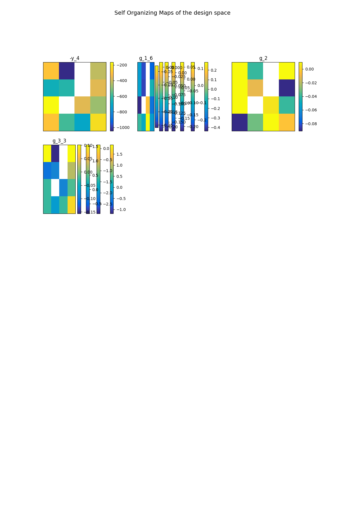
Out:
INFO - 10:03:13: Building Self Organizing Map from optimization history:
INFO - 10:03:13:     Number of neurons in x direction = 4
INFO - 10:03:13:     Number of neurons in y direction = 4
Figure SOM example on the Sobieski problem. illustrates another SOM on the Sobieski
use case. The optimization method is a (costly) derivative free algorithm
(NLOPT_COBYLA), indeed all the relevant information for the optimization
is obtained at the cost of numerous evaluations of the functions. For
more details, please read the paper by
[KJO+06] on wing MDO post-processing
using SOM.
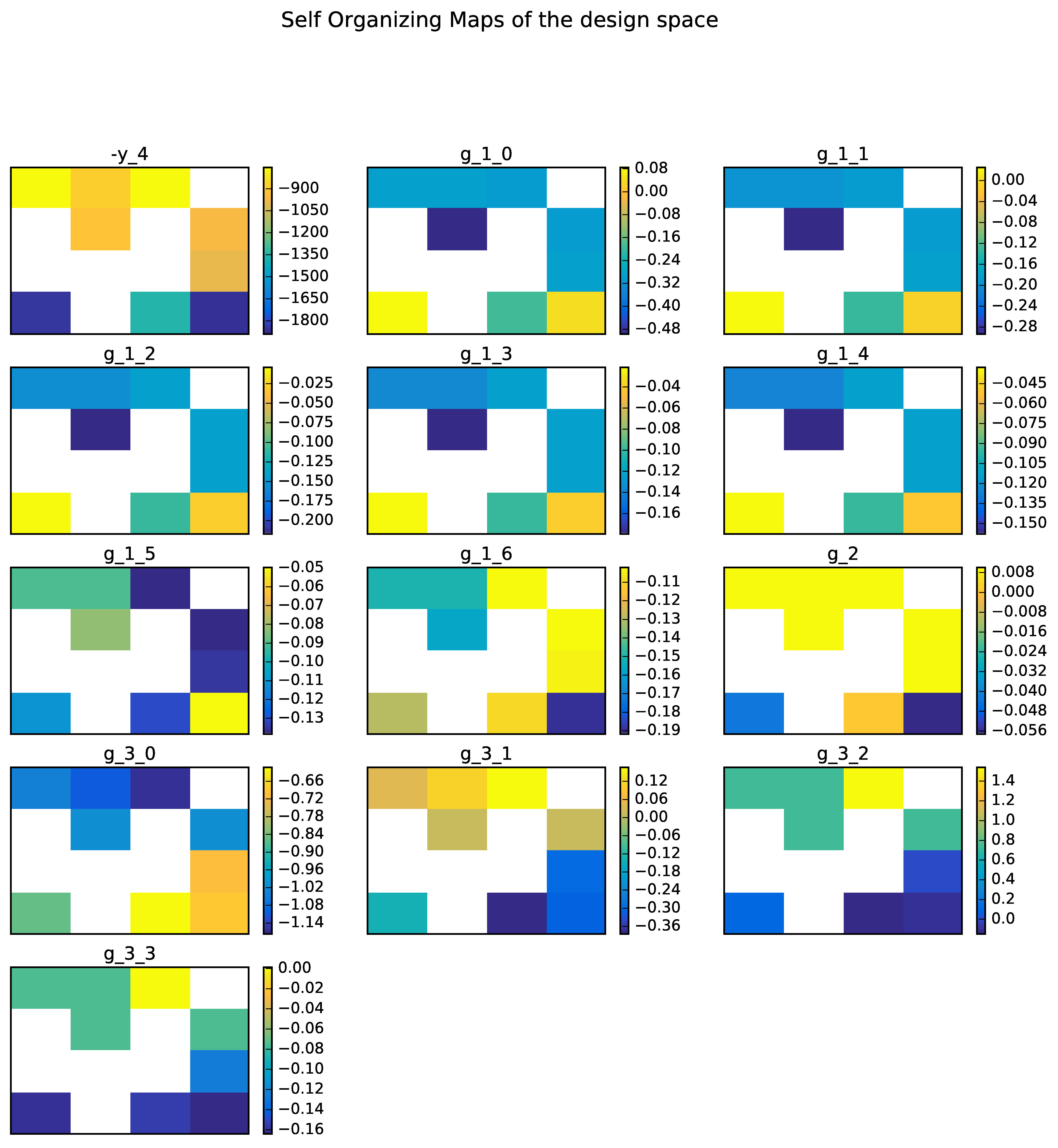
SOM example on the Sobieski problem.
A DOE may also be a good way to produce SOM maps. Figure SOM example on the Sobieski problem with a 10 000 samples DOE. shows an example with 10000 points on the same test case. This produces more relevant SOM plots.
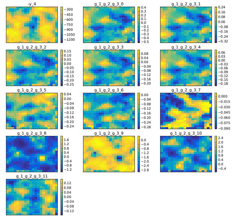
SOM example on the Sobieski problem with a 10 000 samples DOE.
Total running time of the script: ( 0 minutes 2.407 seconds)