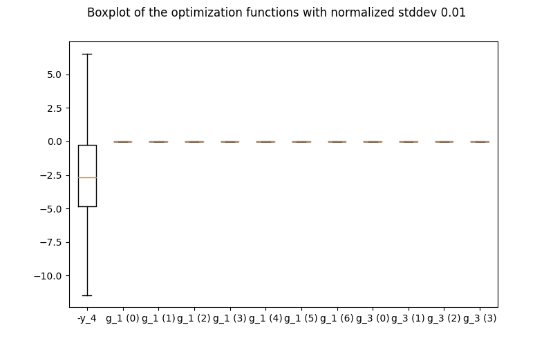
Robustness

In this example, we illustrate the use of the Robustness plot on the Sobieski’s SSBJ problem.

from gemseo.api import configure_logger
from gemseo.api import create_discipline
from gemseo.api import create_scenario
from gemseo.problems.sobieski.core.problem import SobieskiProblem
from matplotlib import pyplot as plt

Import

The first step is to import some functions from the API and a method to get the design space.

configure_logger()

Out:

<RootLogger root (INFO)>

Description

In the Robustness post-processing, the robustness of the optimum is represented by a box plot. Using the quadratic approximations of all the output functions, we propagate analytically a normal distribution with 1% standard deviation on all the design variables, assuming no cross-correlations of inputs, to obtain the mean and standard deviation of the resulting normal distribution. A series of samples are randomly generated from the resulting distribution, whose quartiles are plotted, relatively to the values of the function at the optimum. For each function (in abscissa), the plot shows the extreme values encountered in the samples (top and bottom bars). Then, 95% of the values are within the blue boxes. The average is given by the red bar.

Create disciplines

At this point, we instantiate the disciplines of Sobieski’s SSBJ problem: Propulsion, Aerodynamics, Structure and Mission

disciplines = create_discipline(
    [
        "SobieskiPropulsion",
        "SobieskiAerodynamics",
        "SobieskiStructure",
        "SobieskiMission",
    ]
)

Create design space

We also read the design space from the SobieskiProblem.

design_space = SobieskiProblem().design_space

Create and execute scenario

The next step is to build an MDO scenario in order to maximize the range, encoded ‘y_4’, with respect to the design parameters, while satisfying the inequality constraints ‘g_1’, ‘g_2’ and ‘g_3’. We can use the MDF formulation, the SLSQP optimization algorithm and a maximum number of iterations equal to 100.

scenario = create_scenario(
    disciplines,
    formulation="MDF",
    objective_name="y_4",
    maximize_objective=True,
    design_space=design_space,
)
scenario.set_differentiation_method("user")
for constraint in ["g_1", "g_2", "g_3"]:
    scenario.add_constraint(constraint, "ineq")
scenario.execute({"algo": "SLSQP", "max_iter": 10})

Out:

    INFO - 10:03:04:
    INFO - 10:03:04: *** Start MDOScenario execution ***
    INFO - 10:03:04: MDOScenario
    INFO - 10:03:04:    Disciplines: SobieskiPropulsion SobieskiAerodynamics SobieskiStructure SobieskiMission
    INFO - 10:03:04:    MDO formulation: MDF
    INFO - 10:03:04: Optimization problem:
    INFO - 10:03:04:    minimize -y_4(x_shared, x_1, x_2, x_3)
    INFO - 10:03:04:    with respect to x_1, x_2, x_3, x_shared
    INFO - 10:03:04:    subject to constraints:
    INFO - 10:03:04:       g_1(x_shared, x_1, x_2, x_3) <= 0.0
    INFO - 10:03:04:       g_2(x_shared, x_1, x_2, x_3) <= 0.0
    INFO - 10:03:04:       g_3(x_shared, x_1, x_2, x_3) <= 0.0
    INFO - 10:03:04:    over the design space:
    INFO - 10:03:04:    +----------+-------------+-------+-------------+-------+
    INFO - 10:03:04:    | name     | lower_bound | value | upper_bound | type  |
    INFO - 10:03:04:    +----------+-------------+-------+-------------+-------+
    INFO - 10:03:04:    | x_shared |     0.01    |  0.05 |     0.09    | float |
    INFO - 10:03:04:    | x_shared |    30000    | 45000 |    60000    | float |
    INFO - 10:03:04:    | x_shared |     1.4     |  1.6  |     1.8     | float |
    INFO - 10:03:04:    | x_shared |     2.5     |  5.5  |     8.5     | float |
    INFO - 10:03:04:    | x_shared |      40     |   55  |      70     | float |
    INFO - 10:03:04:    | x_shared |     500     |  1000 |     1500    | float |
    INFO - 10:03:04:    | x_1      |     0.1     |  0.25 |     0.4     | float |
    INFO - 10:03:04:    | x_1      |     0.75    |   1   |     1.25    | float |
    INFO - 10:03:04:    | x_2      |     0.75    |   1   |     1.25    | float |
    INFO - 10:03:04:    | x_3      |     0.1     |  0.5  |      1      | float |
    INFO - 10:03:04:    +----------+-------------+-------+-------------+-------+
    INFO - 10:03:04: Solving optimization problem with algorithm SLSQP:
    INFO - 10:03:04: ...   0%|          | 0/10 [00:00<?, ?it]
    INFO - 10:03:04: ...  20%|██        | 2/10 [00:00<00:00, 41.35 it/sec, obj=-2.12e+3]
    INFO - 10:03:04: ...  30%|███       | 3/10 [00:00<00:00, 24.85 it/sec, obj=-3.15e+3]
    INFO - 10:03:04: ...  40%|████      | 4/10 [00:00<00:00, 17.72 it/sec, obj=-3.96e+3]
    INFO - 10:03:04: ...  50%|█████     | 5/10 [00:00<00:00, 13.77 it/sec, obj=-3.98e+3]
    INFO - 10:03:05: ...  50%|█████     | 5/10 [00:00<00:00, 12.40 it/sec, obj=-3.98e+3]
    INFO - 10:03:05: Optimization result:
    INFO - 10:03:05:    Optimizer info:
    INFO - 10:03:05:       Status: 8
    INFO - 10:03:05:       Message: Positive directional derivative for linesearch
    INFO - 10:03:05:       Number of calls to the objective function by the optimizer: 6
    INFO - 10:03:05:    Solution:
    INFO - 10:03:05:       The solution is feasible.
    INFO - 10:03:05:       Objective: -3960.1367790933214
    INFO - 10:03:05:       Standardized constraints:
    INFO - 10:03:05:          g_1 = [-0.01805983 -0.03334555 -0.04424879 -0.05183405 -0.05732561 -0.13720865
    INFO - 10:03:05:  -0.10279135]
    INFO - 10:03:05:          g_2 = 2.9360600315442298e-06
    INFO - 10:03:05:          g_3 = [-0.76310174 -0.23689826 -0.00553375 -0.183255  ]
    INFO - 10:03:05:       Design space:
    INFO - 10:03:05:       +----------+-------------+---------------------+-------------+-------+
    INFO - 10:03:05:       | name     | lower_bound |        value        | upper_bound | type  |
    INFO - 10:03:05:       +----------+-------------+---------------------+-------------+-------+
    INFO - 10:03:05:       | x_shared |     0.01    | 0.06000073401500788 |     0.09    | float |
    INFO - 10:03:05:       | x_shared |    30000    |        60000        |    60000    | float |
    INFO - 10:03:05:       | x_shared |     1.4     |         1.4         |     1.8     | float |
    INFO - 10:03:05:       | x_shared |     2.5     |         2.5         |     8.5     | float |
    INFO - 10:03:05:       | x_shared |      40     |          70         |      70     | float |
    INFO - 10:03:05:       | x_shared |     500     |         1500        |     1500    | float |
    INFO - 10:03:05:       | x_1      |     0.1     |         0.4         |     0.4     | float |
    INFO - 10:03:05:       | x_1      |     0.75    |         0.75        |     1.25    | float |
    INFO - 10:03:05:       | x_2      |     0.75    |         0.75        |     1.25    | float |
    INFO - 10:03:05:       | x_3      |     0.1     |  0.1553801266337427 |      1      | float |
    INFO - 10:03:05:       +----------+-------------+---------------------+-------------+-------+
    INFO - 10:03:05: *** End MDOScenario execution (time: 0:00:00.819730) ***

{'max_iter': 10, 'algo': 'SLSQP'}

Post-process scenario

Lastly, we post-process the scenario by means of the Robustness which plots any of the constraint or objective functions w.r.t. the optimization iterations or sampling snapshots.

Tip

Each post-processing method requires different inputs and offers a variety of customization options. Use the API function get_post_processing_options_schema() to print a table with the options for any post-processing algorithm. Or refer to our dedicated page: Post-processing algorithms.

scenario.post_process("Robustness", save=False, show=False)
# Workaround for HTML rendering, instead of ``show=True``
plt.show()