Probability distributions based on OpenTURNS

In this example, we seek to create a probability distribution based on the OpenTURNS library.

from __future__ import annotations

from gemseo import configure_logger
from gemseo.uncertainty import create_distribution
from gemseo.uncertainty import get_available_distributions

configure_logger()

<RootLogger root (INFO)>

First of all, we can access the names of the available probability distributions from the API:

all_distributions = get_available_distributions()
all_distributions

['OTComposedDistribution', 'OTDiracDistribution', 'OTDistribution', 'OTExponentialDistribution', 'OTNormalDistribution', 'OTTriangularDistribution', 'OTUniformDistribution', 'OTWeibullDistribution', 'SPComposedDistribution', 'SPDistribution', 'SPExponentialDistribution', 'SPNormalDistribution', 'SPTriangularDistribution', 'SPUniformDistribution', 'SPWeibullDistribution']

and filter the ones based on the OpenTURNS library (their names start with the acronym ‘OT’):

ot_distributions = get_available_distributions("OTDistribution")
ot_distributions

['OTDiracDistribution', 'OTDistribution', 'OTExponentialDistribution', 'OTNormalDistribution', 'OTTriangularDistribution', 'OTUniformDistribution', 'OTWeibullDistribution']

Create a distribution

Then, we can create a probability distribution for a two-dimensional random variable with independent components that follow a normal distribution.

Case 1: the OpenTURNS distribution has a GEMSEO class

For the standard normal distribution (mean = 0 and standard deviation = 1):

distribution_0_1 = create_distribution("x", "OTNormalDistribution", 2)
distribution_0_1

Normal[2](mu=0.0, sigma=1.0)

For a normal with mean = 1 and standard deviation = 2:

distribution_1_2 = create_distribution(
    "x", "OTNormalDistribution", 2, mu=1.0, sigma=2.0
)
distribution_1_2

Normal[2](mu=1.0, sigma=2.0)

Case 2: the OpenTURNS distribution has no GEMSEO class

When GEMSEO does not offer a class for the OpenTURNS distribution, we can use the generic GEMSEO class OTDistribution to create any OpenTURNS distribution by setting interfaced_distribution to its OpenTURNS name and parameters as a tuple of OpenTURNS parameter values (see the documentation of OpenTURNS).

distribution_1_2 = create_distribution(
    "x", "OTDistribution", 2, interfaced_distribution="Normal", parameters=(1.0, 2.0)
)
distribution_1_2

Normal[2](1.0, 2.0)

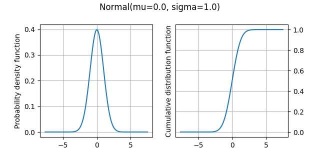
Plot the distribution

We can plot both cumulative and probability density functions for the first marginal:

distribution_0_1.plot()

<Figure size 640x320 with 2 Axes>

Note

We can provide a marginal index as first argument of the Distribution.plot() method but in the current version of GEMSEO, all components have the same distributions and so the plot will be the same.

Get statistics

Mean

We can access the mean of the distribution:

distribution_0_1.mean

array([0., 0.])

Standard deviation

We can access the standard deviation of the distribution:

distribution_0_1.standard_deviation

array([1., 1.])

Numerical range

We can access the range, i.e. the difference between the numerical minimum and maximum, of the distribution:

distribution_0_1.range

[array([-7.65062809,  7.65062809]), array([-7.65062809,  7.65062809])]

Mathematical support

We can access the range, i.e. the difference between the minimum and maximum, of the distribution:

distribution_0_1.support

[array([-inf,  inf]), array([-inf,  inf])]

Compute CDF

We can compute the cumulative density function component per component (here the probability that the first component is lower than 0. and that the second one is lower than 1.):

distribution_0_1.compute_cdf([0.0, 1.0])

array([0.5       , 0.84134475])

Compute inverse CDF

We can compute the inverse cumulative density function component per component (here the quantile at 50% for the first component and the quantile at 97.5% for the second one):

distribution_0_1.compute_inverse_cdf([0.5, 0.975])

array([0.        , 1.95996398])

Generate samples

We can generate 10 samples of the distribution:

distribution_0_1.compute_samples(10)

array([[ 0.60820165, -0.4705256 ],
       [-1.2661731 ,  0.26101794],
       [-0.43826562, -2.29006198],
       [ 1.2054782 , -1.28288529],
       [-2.18138523, -1.31178112],
       [ 0.35004209, -0.09078383],
       [-0.35500705,  0.99579323],
       [ 1.43724931, -0.13945282],
       [ 0.81066798, -0.5602056 ],
       [ 0.79315601,  0.4454897 ]])